H3 indexes for performance with PostGIS data

I recently started using the H3 hex grid extension in Postgres with the goal of making some not-so-fast queries faster. My previous post, Using Uber's H3 hex grid in PostGIS, has an introduction to the H3 extension. The focus in that post, admittedly, is a PostGIS focused view instead of an H3 focused view. This post takes a closer look at using the H3 extension to enhance performance of spatial searches.

The two common spatial query patterns considered in this post are:

• Nearest neighbor style searches
• Regional analysis

This post used the H3 v3 extension. See Using v4 of the Postgres H3 extension for usage in the latest version.

Setup and Point of Focus

This post uses two tables to examine performance. The following queries add an h3_ix column to the osm.natural_point and osm.building_polygon tables. This approach uses GENERATED columns and adds an index to the column. Going through these steps allow us to remove the need for PostGIS joins at query time for rough distance searches. See my previous post for details about installing the H3 extension and the basics of how it works.

The data used in this post is Colorado OpenStreetMap data loaded using PgOSM Flex.

First, add the H3 index to the osm.natural_point table. It takes about 3 seconds to calculate the H3 index and create an index on the osm.natural_point table.

ALTER TABLE osm.natural_point ADD h3_ix H3INDEX
    GENERATED ALWAYS AS (
        h3_geo_to_h3(ST_Transform(geom, 4326), 7)
    ) STORED
;
CREATE INDEX gix_natural_point_h3_ix
    ON osm.natural_point (h3_ix);

To create the H3 index on the osm.building_polygon table we need to add the ST_Centroid() step into the definition. It takes about 12 seconds to run these steps on the building polygon table.

ALTER TABLE osm.building_polygon ADD h3_ix H3INDEX
    GENERATED ALWAYS AS (
        h3_geo_to_h3(ST_Transform(ST_Centroid(geom), 4326), 7)
    ) STORED
;
CREATE INDEX gix_building_polygon_h3_ix
    ON osm.building_polygon (h3_ix);

The H3 indexes are now calculated for these two tables. My next step is to pick a building to use for a point of focus for the coming spatial search examples. I select a building, Pangea Coffee Roasters, in Golden, Colorado using its osm_id. The following query returns the h3_ix, the point is shown on the map in the following screenshot.

SELECT osm_id, name, h3_ix, geom
    FROM osm.building_polygon
    WHERE osm_id = 392853178
;

┌───────────┬────────────────────────┬─────────────────┐
│  osm_id   │          name          │      h3_ix      │
╞═══════════╪════════════════════════╪═════════════════╡
│ 392853178 │ Pangea Coffee Roasters │ 872681364ffffff │
└───────────┴────────────────────────┴─────────────────┘

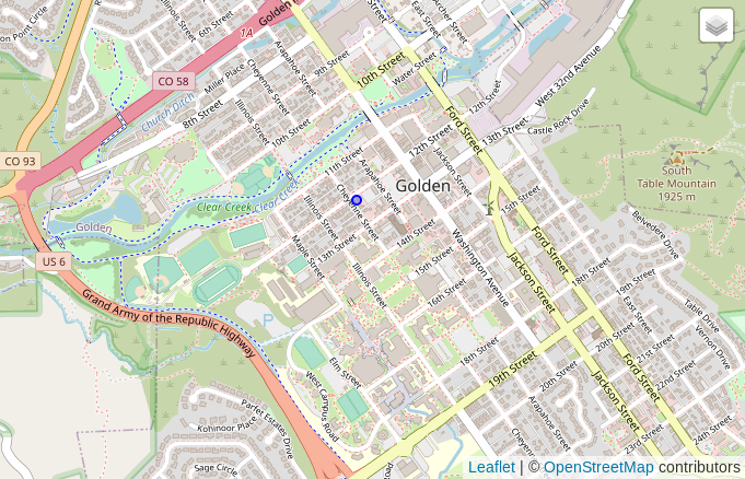
The query above returned the h3_ix value (872681364ffffff) for the resolution 7 hex containing Pangea Coffee Roasters. We can see the polygon of the hex using the h3_to_geo_boundary_geometry() function.

SELECT h3_to_geo_boundary_geometry('872681364ffffff');

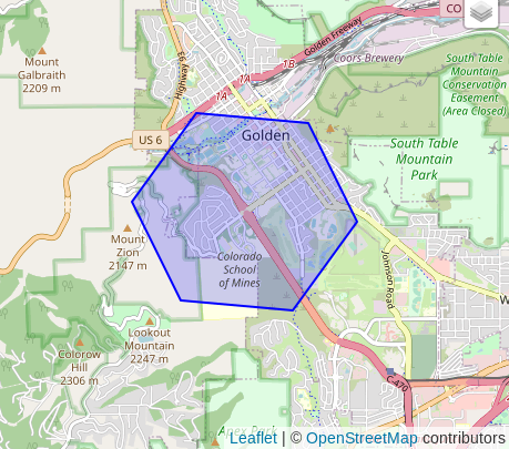
Using H3's grid traversal functions it is easy to find a basic relationship between the number of rings of hexagons and the size of radius. The following query uses the h3_k_ring() function to include 3 rings of hexes surrounding the hex of focus (872681364ffffff). It just so happens, that this 3-ring hex buffer roughly lines up with a 10 kilometer buffer calculated using SRID 3857. The 10 km buffer is also shown for comparison.

-- Resolution 7, looking out 3 rings -- Roughly 10 km radius!
SELECT b.osm_id,
        ST_Buffer(b.geom, 10000) AS buffer_10km,
        b.geom,
        h3_to_geo_boundary_geometry(
            h3_k_ring(h3_geo_to_h3(ST_Transform(b.geom, 4326), 7), 3)
            ) AS ix_ring
    FROM osm.vbuilding_all b
    WHERE b.osm_id = 392853178
;

The h3_k_ring() is one of many functions offered by the H3 index. Check out the full API reference for a look at the rest of the functionality.

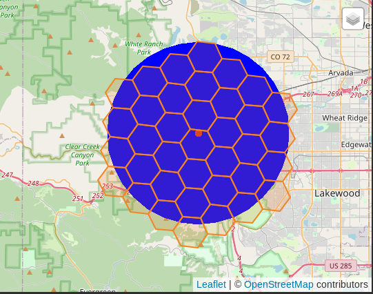
To get a radius 4 times larger we can multiply both values by 4 to use a 40 km buffer and a 12-ring hex buffer in h3_k_ring() function. This results in a grid of 469 hexagons.

-- Looking out 3*4 (12) rings -- Roughly 10*4 km (40km) radius!
SELECT b.osm_id,
        ST_Buffer(b.geom, 10000*4) AS buffer_10km,
        b.geom,
        h3_to_geo_boundary_geometry(
            h3_k_ring(h3_geo_to_h3(ST_Transform(b.geom, 4326), 7), 3*4)
            ) AS ix_ring
    FROM osm.vbuilding_all b
    WHERE b.osm_id = 392853178
;

The above examples show that I was able to quickly establish a rough relationship between a measurement we know (10 km) with a more abstract measurement (3 hex rings at resolution 7). It is helpful for us humans and usability to have a somewhat familiar frame of reference.

Nearest Neighbor Style Searches

This example uses PostGIS's ST_DWithin() function to find trees within 10 kilometers from the focus point. This query with a traditional spatial join takes 14 - 25 ms to run. It returns around 12,000 rows.

EXPLAIN (ANALYZE, BUFFERS, VERBOSE, FORMAT JSON)
SELECT b.osm_id, b.name, b.height, n.geom
    FROM osm.building_polygon b
    INNER JOIN osm.natural_point n
        ON n.osm_type = 'tree' AND ST_DWithin(b.geom, n.geom, 10000)
    WHERE b.osm_id = 392853178
;

The query plan visualized by pgMustard shows this query is decently efficient. The following screenshot shows the main overview of the nodes with the total time and the node timings. The GIST index on natural_point was used, taking 8ms of the query time.

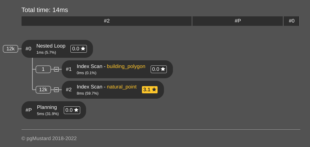
If you look closely at row estimates (open that link to pgMustard!) you'll notice that the estimated rows returned from natural_point was significantly off from the actual number of rows. In the case of this query, it was "out by a factor of 390.4." Spatial joins commonly have poor row estimates used by the query planner and are often the cause of poor spatial query performance.

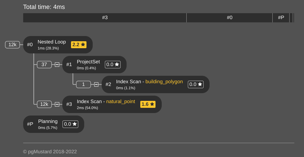
The next query uses the H3 index from the selected building, and passes h3_ix into the h3_k_ring() function. This creates the 3-ring hex buffer to use for the join to the osm.natural_point table, replacing the spatial join. The query with the H3 index is 73% faster, returning in 4 - 6 ms. The query plan shows that two indexes are used again. This query also returns around 12,000 rows.

EXPLAIN (ANALYZE, BUFFERS, VERBOSE, FORMAT JSON)
WITH rng AS (
SELECT h3_k_ring(h3_ix, 3)
            AS ix_ring
    FROM osm.building_polygon b
    WHERE b.osm_id = 392853178
)
SELECT *
    FROM rng b
    INNER JOIN osm.natural_point n
        ON n.osm_type = 'tree'
            AND n.h3_ix = b.ix_ring
;

Increasing result size

This section switches the query to look for buildings within a 40 km radius instead of trees within 10 km. With this change the following queries return roughly 340,000 rows each. The spatial join for with ST_DWithin() and a 40km radius returns in 459 ms. Using a 12-ring hex buffer returns in about 100 ms, 78% faster.

SELECT b.osm_id, b.name, b.height, n.geom
    FROM osm.building_polygon b
    INNER JOIN osm.building_polygon n
        ON ST_DWithin(b.geom, n.geom, 10000*4)
    WHERE b.osm_id = 392853178
;

WITH rng AS (
SELECT h3_k_ring(h3_ix, 3*4)
            AS ix_ring
    FROM osm.building_polygon b
    WHERE b.osm_id = 392853178
)
SELECT *
    FROM rng b
    INNER JOIN osm.building_polygon n
        ON n.h3_ix = b.ix_ring
;

Regional Analysis

The queries above use the pattern of finding "those" within "a distance" of "this." This section switches to the a query to answer "show me this pattern across a region" questions. My post Find missing crossings in OpenStreetMap with PostGIS is an example that type of analysis.

Since my test database already has H3 indexes available for trees and buildings, this example calculates the number of trees per building within each hex. The first query uses spatial joins between the feature table and the h3.hex table.

The h3.hex table was created to cover Colorado following the steps I outlined in my previous post under "Save the hexes."

WITH bldgs AS (
SELECT h.ix AS h3_ix, 'building' AS src, COUNT(*) AS cnt
    FROM osm.building_polygon b
    INNER JOIN h3.hex h ON ST_Contains(h.geom_3857, ST_Centroid(b.geom))
    GROUP BY h.ix
), trs AS (
SELECT h.ix AS h3_ix, n.osm_type AS src, COUNT(*) AS cnt
    FROM osm.natural_point n
    INNER JOIN h3.hex h ON ST_Contains(h.geom_3857, n.geom)
    WHERE n.osm_type = 'tree'
    GROUP BY h.ix, n.osm_type
)
SELECT COALESCE(b.h3_ix, t.h3_ix) AS h3_ix,
        CASE WHEN b.cnt > 0
            THEN 1.0 * t.cnt / b.cnt
            ELSE NULL
            END AS tree_per_bldg
    FROM bldgs b
    FULL JOIN trs t ON b.h3_ix = t.h3_ix
;

The next query uses the H3 indexes. By using these indexes, the aggregate queries do not need to know anything about the "where" of the data, only the H3 index. The h3_ix column is basically just a short piece of text.

WITH bldgs AS (
SELECT h3_ix, 'building' AS src, COUNT(*) AS cnt
    FROM osm.building_polygon
    GROUP BY h3_ix
), trs AS (
SELECT h3_ix, osm_type AS src, COUNT(*) AS cnt
    FROM osm.natural_point
    WHERE osm_type = 'tree'
    GROUP BY h3_ix, osm_type
)
SELECT COALESCE(b.h3_ix, t.h3_ix) AS h3_ix,
        CASE WHEN b.cnt > 0
            THEN 1.0 * t.cnt / b.cnt
            ELSE NULL
            END AS tree_per_bldg
    FROM bldgs b
    FULL JOIN trs t ON b.h3_ix = t.h3_ix
;

The query using the spatial join took 22 seconds (query plan).

The query using the H3 indexes took only 182 ms... That's 99% faster! (query plan)

Sum of buffers: measure of work

When looking at the previous query plan using spatial joins in pgMustard, the "Sum of buffers" detail caught my attention. The following screenshot shows a reported 51 GB of buffers used!

I knew the total of the tables involved was well under 1 GB in size. This made me curious, so I asked Michael Christofides, co-founder of pgMustard, what was behind the sum of buffers calculation.

"pgMustard does some arithmetic to calculate (and display) these on a per node basis, in the Buffers section. It also now a works out roughly how much data each of them represents in kB/MB/GB/TB, assuming an 8kB block size.

The sum is simply a crude addition of all of these per-node numbers put together! Naturally blocks can be read more than once for the same query, and reads and writes to disk are double counted, but since I see it as a very rough measure of “work done”, I thought the sum worked surprisingly well. It’s not perfect, and I still focus more on timings, but I think it helps folks understand why some things are slower than they expected!" -- Michael Christofides

Admittedly, the total number by itself threw me off at first. After looking at this value on a number of query plans, it has grown on me! It seems to be a decent indicator how much data a query is using and that is a good thing to have an eye on. Another great addition to an already solid tool.

Summary

This post has explored using the H3 extension in Postgres, with the goal of improving performance for specific types of spatial queries.

• Nearest neighbor style searches
• Regional analysis

The two queries I tested for the nearest neighbor searches performed 73% - 77% faster with H3 indexes. The regional analysis was 99% faster. These are huge wins, especially as data sizes grow and the complexity of spatial queries increases. It is common to have queries using these patterns that can take a few minutes to run. Cutting out 70-99% of the query time sounds good to me!

Need help with your PostgreSQL servers or databases? Contact us to start the conversation!