Using Uber's H3 hex grid in PostGIS

This post explores using the H3 hex grid system within PostGIS. H3 was developed by Uber and has some cool benefits over the PostGIS native ST_HexagonGrid() function used in my post Find missing crossings in OpenStreetMap with PostGIS. The hex grid built-in to PostGIS is great for one-off projects covering a specific region, though it has shortcomings for larger scale consistency. On the other hand, the H3 grid is a globally defined grid that scales up and down through resolutions neatly. For more details, read Uber's description.

This post used the H3 v3 extension. See Using v4 of the Postgres H3 extension for usage in the latest version.

This post works through a few of the functions available in the H3 extension and how they can be used for spatial aggregation in an analysis. One additional focus is how to generate a table of H3 hexagons for a given resolution.

Note: This post does not focus on using H3 for the best performance. See my post H3 indexes for performance with PostGIS data for a look into high performance spatial searches with H3.

Install H3 in Postgres

The H3 library is available to PostGIS as a Postgres extension. I am using the bytesandbrains h3-pg project available on GitHub. The extension can be installed using pgxn install h3. Once installed, create the H3 extension in the database.

CREATE EXTENSION h3;

First Steps

With the extension installed, I found the project's API reference to be a helpful starting point. This helped me to start understanding how the various functions work and determining what was possible.

H3 uses 16 resolutions (zoom level) from 0 to 15. The Table of Cell Areas for H3 Resolutions shows these resolutions with average size details and the number of unique indexes (hexagons) in that resolution. Resolution 0 is the largest scale with only 122 hexagons for the entire globe. Resolution 6 starts getting decently large (14 million hexagons) and resolution 15 is large by all means, with nearly 570 trillion hexagons. For the scale of my use cases, resolutions 5 through 8 end up being the most helpful to me.

The H3 extension comes with a h3_num_hexagons(resolution int4) function that also provides the hexagon counts for a given resolution.

SELECT i, h3_num_hexagons(i)
    FROM generate_series(0, 15, 3) i
;

┌────┬─────────────────┐
│ i  │ h3_num_hexagons │
╞════╪═════════════════╡
│  0 │             122 │
│  3 │           41162 │
│  6 │        14117882 │
│  9 │      4842432842 │
│ 12 │   1660954464122 │
│ 15 │ 569707381193162 │
└────┴─────────────────┘

The generate_series() function is useful in so many ways!

Index from geometry

With a database full of OpenStreetMap data loaded via PgOSM Flex, my next step is to grab some data and see what H3 index it is in. The h3_geo_to_h3 function does exactly this. A couple caveats to point out:

• Only works on points
• Must be in SRID 4326

I found the first caveat because one of my most commonly used tables from the OSM data is osm.road_line. Attempting to pass in the line data to the h3_geo_to_h3() function results in an error.

ERROR: geometry_to_point only accepts Points

The following query selects a single road segment, transforms it to SRID 4326, calculates the centroid and determines the hex index for resolution 6.

SELECT h3_geo_to_h3(
            ST_Centroid(ST_Transform(geom, 4326)), 6)
    FROM osm.road_line
    WHERE osm_id = 289242317
;

┌─────────────────┐
│  h3_geo_to_h3   │
╞═════════════════╡
│ 862681ac7ffffff │
└─────────────────┘

The H3 index is a big part of what makes the really cool stuff work, but for now all I want to see the geometry. This visual step is critical for me to help verify it is working the way I assume it is. It wasn't until I ran this step with h3_to_geo_boundary_geometry() that I realized that the ST_Transform() was required, as my default geometry data is in SRID 3857.

SELECT h3_to_geo_boundary_geometry(
        h3_geo_to_h3(
            ST_Centroid(ST_Transform(geom, 4326)), 6)), *
    FROM osm.road_line
    WHERE osm_id = 289242317
;

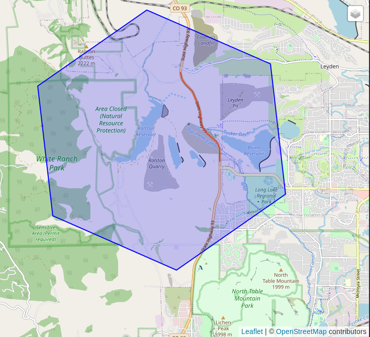
Assigning long lines to a hex based on only its centroid may work for some use cases, while others may need to calculate the hex for individual nodes within the line for best results. The image above shows that at resolution 6, the selected line fits entirely within a single hexagon.

Save the hexes

The prior example showed how existing geometry data can be assigned to an H3 hex. While many examples using H3 will be most interested in that type of operation coupled with nearest neighbor style searches, I really wanted to get to the point where I could create a grid of hexes, similar to Step 2 in this post that used ST_HexagonGrid(). There are a couple reasons I want a table of H3 hexes.

First, I want to be able to run a spatial analysis and find areas where something is entirely missing. Queries with the H3 functions/indexes seem to be good at telling me "where things are" (this geom is in that index) but I didn't see an obvious way to find the areas where "this thing is not." With a table of hexes, that's an easy solution with a LEFT JOIN. The final query in this post is an example of that use case.

Another reason this is helpful is because not every PostGIS enabled system can install the H3 extension. Managed database services, such as AWS RDS or MS Azure, do not seem to support this extension yet. Also, some organizations have strict policies related to adding new software to production systems. Being able to save the data needed into table format allows using the H3 hexagons without the requirement of the H3 extension.

I create an h3 schema and create a table in it to store the hexagons. The ix column uses the h3index type as the primary key.

CREATE SCHEMA h3;
CREATE TABLE h3.hex
(
    ix H3INDEX NOT NULL PRIMARY KEY,
    resolution INT2 NOT NULL,
    geom GEOMETRY (POLYGON, 4326) NOT NULL,
    CONSTRAINT ck_resolution CHECK (resolution >= 0 AND resolution <= 15)
);
CREATE INDEX gix_h3_hex ON h3.hex USING GIST (geom);

Note: If you plan to use this table in a database without the H3 extension you will not be able to use the h3index data type. Casting the data to TEXT should work, though potentially has additional caveats not explored in this post.

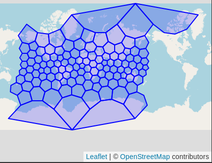
The function h3_get_res_0_indexes() provides our starting point by returning the 122 hexagons at resolution 0. This function along with h3_to_geo_boundary_geometry() again is used to INSERT data into the h3.hex table.

INSERT INTO h3.hex (ix, resolution, geom)
SELECT ix, 0 AS resolution,
        h3_to_geo_boundary_geometry(ix, True) AS geom
    FROM h3_get_res_0_indexes() ix
;

A quick count query verifies the 122 hexagons.

SELECT resolution, COUNT(*)
    FROM h3.hex
    GROUP BY resolution
;

┌────────────┬──────────┐
│ resolution │  count   │
╞════════════╪══════════╡
│          0 │      122 │
└────────────┴──────────┘

The resulting hexagons look like the following screenshot from DBeaver's spatial viewer.

With the resolution 0 hexes created, they can now be used to generate one level higher. The next query uses the understanding that one parent hex relates to seven (7) children hexes. It also introduces two more H3 functions: h3_to_center_child() and h3_k_ring().

"H3 supports sixteen resolutions. Each finer resolution has cells with one seventh the area of the coarser resolution. Hexagons cannot be perfectly subdivided into seven hexagons, so the finer cells are only approximately contained within a parent cell." -- Isaac Brodsky

The h3_to_center_child() identifies the hexagon in the next resolution at the center of the given index (ix). The h3_k_ring() function grabs the six (6) hexes surrounding that center child.

INSERT INTO h3.hex (ix, resolution, geom)
SELECT h3_k_ring(h3_to_center_child(ix)) AS ix,
        resolution + 1 AS resolution,
        h3_to_geo_boundary_geometry(h3_k_ring(h3_to_center_child(ix)), True)
            AS geom
    FROM h3.hex 
    WHERE resolution IN (SELECT MAX(resolution) FROM h3.hex)
;

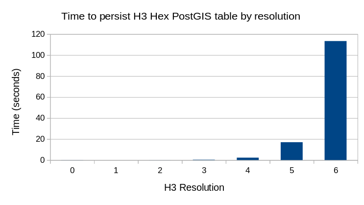
The where clause in this query is setup to make this a lazy process, though this will not be the fastest performing query with the nested query in the where clause. If you want resolution 6, run this query 6 times. Be aware that the time to create each subsequent resolution increases exponentially.

The row counts and timings below were taken from persisting resolutions 1 through 6. Resolution 4 took 2.3 seconds to insert, resolution 5 took 17 seconds, and 6 took nearly 2 minutes.

INSERT 0 842
Time: 10.509 ms

INSERT 0 5882
Time: 45.755 ms

INSERT 0 41162
Time: 343.010 ms

INSERT 0 288122
Time: 2300.410 ms (00:02.300)

INSERT 0 2016842
Time: 16993.390 ms (00:16.993)

INSERT 0 14117882
Time: 113363.480 ms (01:53.363)

These timings are visualized in the following chart. The timings for resolutions 0 - 2 do not even show up as visible on this chart.

Focused hexes

Creating and saving the full grid for each resolution across the globe is not beneficial. By the time you get to resolution 9 you are looking at 4.8 billion rows for the entire globe. For the more detailed hexes I use, I will limit the scope of the hexes to the area of analysis.

The following series of queries starts by using the h3.hex data for resolution 4 to create hexes covering the polygon of Denver, Colorado. It starts by mimicking the h3.hex table in a new h3.hex_denver table.

CREATE TABLE h3.hex_denver (LIKE h3.hex INCLUDING ALL);

The initial INSERT statement generates resolution 5 starting from resolution 4 in the h3.hex table. The query joins a table osm_denver.focus that has a single row containing the boundary of Denver.

INSERT INTO h3.hex_denver (ix, resolution, geom)
SELECT h3_k_ring(h3_to_center_child(h.ix)) AS ix,
        h.resolution + 1 AS resolution,
        h3_to_geo_boundary_geometry(h3_k_ring(h3_to_center_child(h.ix)), True)
            AS geom
    FROM h3.hex h
    INNER JOIN osm_denver.focus f ON h.geom && ST_Transform(f.geom, 4326)
    WHERE h.resolution = 4
;

Now build subsequent levels from the Denver hexes. This again uses a subquery to determine the next resolution, and defines the join using ST_Intersects(). Again, run this query once for each additional resolution you wish to save.

INSERT INTO h3.hex_denver (ix, resolution, geom)
SELECT h3_k_ring(h3_to_center_child(h.ix)) AS ix,
        h.resolution + 1 AS resolution,
        h3_to_geo_boundary_geometry(h3_k_ring(h3_to_center_child(h.ix)), True)
            AS geom
    FROM h3.hex_denver h
    INNER JOIN osm_denver.focus f
        ON ST_Intersects(h.geom, ST_Transform(f.geom, 4326))
    WHERE resolution IN (SELECT MAX(resolution) FROM h3.hex_denver)
;

Level 10 for the area of the Denver polygon is 27,538 hexagons, created in just over 3 seconds.

INSERT 0 27538
Time: 3110.836 ms (00:03.111)

A quick look at counts by resolution in the h3.hex_denver table.

SELECT resolution, COUNT(*)
    FROM h3.hex_denver
    GROUP BY resolution
    ORDER BY resolution
;

┌────────────┬───────┐
│ resolution │ count │
╞════════════╪═══════╡
│          5 │    28 │
│          6 │    42 │
│          7 │   175 │
│          8 │   840 │
│          9 │  4515 │
│         10 │ 27538 │
└────────────┴───────┘

Visualize OpenStreetMap data

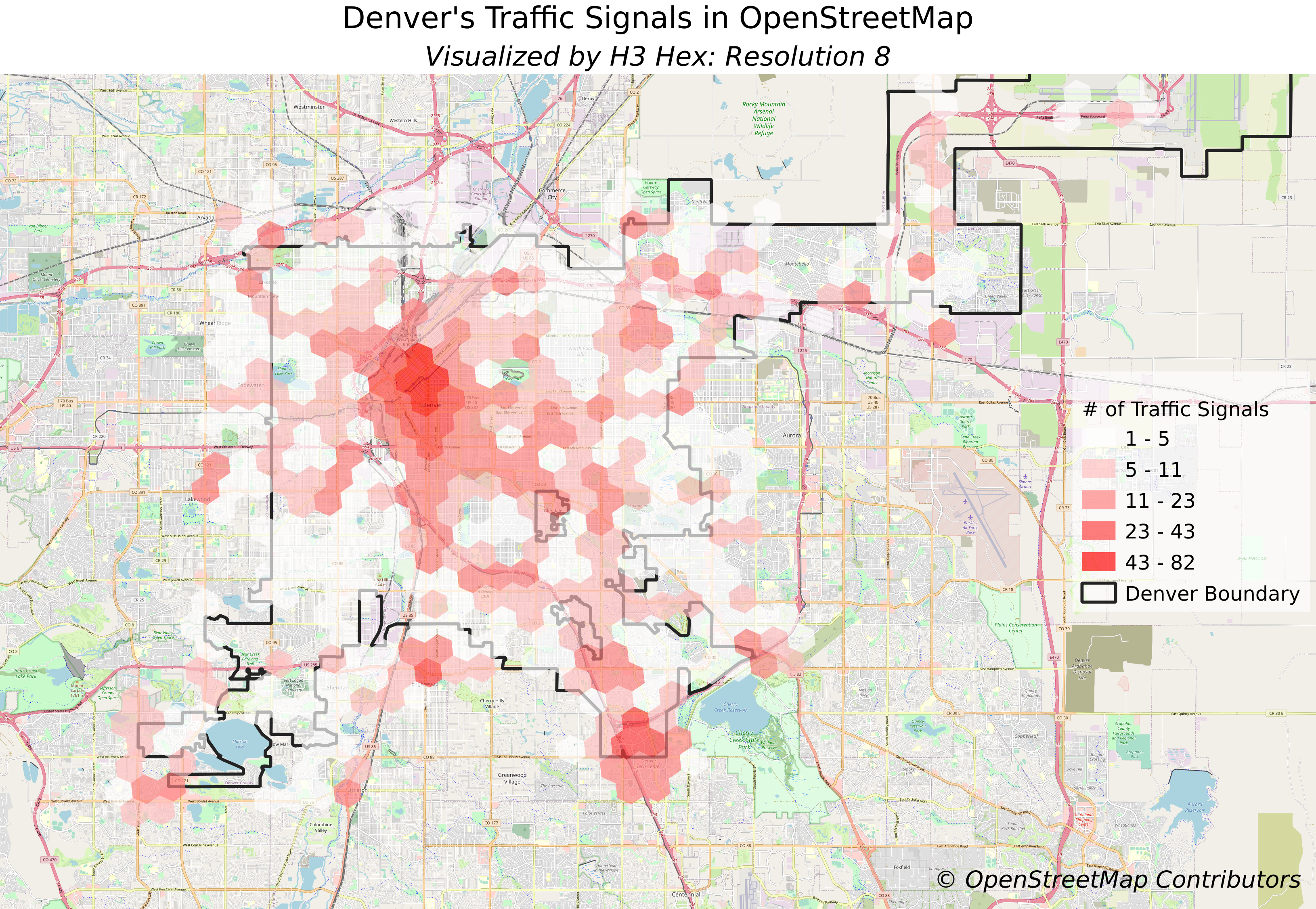
To show how these hexagons can now be used, the following query joins the Denver hexagons to a table osm.traffic_point with traffic signals from OpenStreetMap. The result of the query is saved to h3.hex_denver_traffic_signals to make the styling work in QGIS faster.

DROP TABLE IF EXISTS h3.hex_denver_traffic_signals;
CREATE TABLE h3.hex_denver_traffic_signals AS
SELECT h.ix, h.geom, COUNT(t.osm_id) AS cnt
    FROM h3.hex_denver h
    LEFT JOIN osm.traffic_point t
        ON ST_Transform(t.geom, 4326) && h.geom
            AND t.osm_type = 'traffic_signals'    
    WHERE h.resolution = 8
    GROUP BY h.ix, h.geom
;

The query is not terribly slow (~ 1-2 seconds) but that execution time plus network (server in New York, I'm in Colorado), and rendering makes it worthwhile to just save the data into a table.

The map below was created in QGIS with a filter for cnt > 0. The map clearly shows the traffic signal density in the heart of Denver. It also shows some gaps in the middle of urban areas. Those gaps almost certainly have stoplights in real life, they just had not been digitized into OpenStreetMap when this data set was loaded to PostGIS.

Summary

The H3 library is a powerful extension available to add into Postgres and PostGIS. This post covered a few essential functions in the H3 extension. It also covered a simple approach to put the H3 hexagon data into a familiar format to PostGIS users: a table with spatial data! When it comes time to share the results of spatial analysis, this allows exporting results without the hexagon geometry data, relying on the H3 index.

The examples here barely scratch the surface of H3's capability, and does not even breach the topic of the potential performance benefits using the H3 indexes. Stay tuned for more!

Need help with your PostgreSQL servers or databases? Contact us to start the conversation!