Find missing crossings in OpenStreetMap with PostGIS

The #30DayMapChallenge is going on again this November. Each day of the month has a different theme for that day's map challenge. These challenges do not have a requirement for technology, so naturally I am using OpenStreetMap data stored in PostGIS with QGIS for the visualization component.

The challenge for Day 5 was an OpenStreetMap data challenge. I decided to find and visualize missing crossing tags. Crossing tags are added to the node (point) where a pedestrian highway (e.g. highway=footway) intersects a motorized highway (e.g. highway=tertiary). This post explains how I used PostGIS and OpenStreetMap data to find intersections missing a dedicated crossing tag.

Without further ado, here was my submission for Day 5.

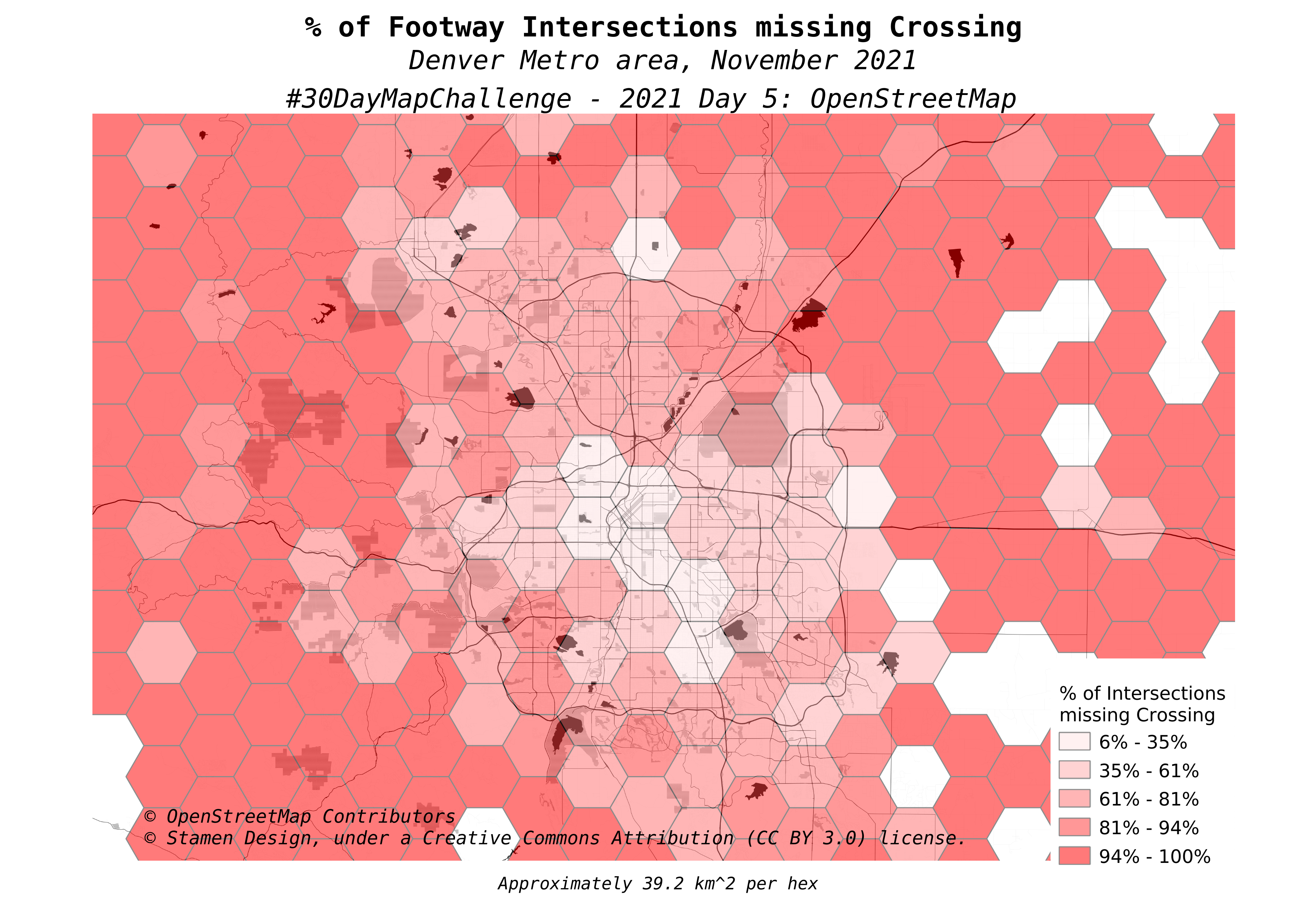
If you're here for the maps, there are four more maps near the bottom under "More Maps." The bulk of this post explains how I got the data to create this visualization.

Step 1: Load data

These days when I load OpenStreetMap data to PostGIS I use the PgOSM Flex Docker image. The PgOSM Flex project uses osm2pgsql's flex output (see Hands on with osm2pgsql's new Flex output) to prepare high quality OpenStreetMap data for PostGIS. The following instructions are from the main project readme, only adjusted to load Colorado instead of the smaller D.C. region used in those examples.

The Docker container needs a user and password.

export POSTGRES_USER=postgres
export POSTGRES_PASSWORD=doNotUseMeIamAPasswordFromTheInternet

Run the container with the local ~/pgosm-data directory linked to the container's path /app/output. This is where PgOSM Flex will save the data files and the processed output.

docker run --name pgosm -d --rm \
    -v ~/pgosm-data:/app/output \
    -v /etc/localtime:/etc/localtime:ro \
    -e POSTGRES_PASSWORD=$POSTGRES_PASSWORD \
    -p 5433:5432 -d rustprooflabs/pgosm-flex

Load the region of choice (Colorado) with the default layerset. This takes about 7 minutes to run on my laptop.

docker exec -it \
    pgosm python3 docker/pgosm_flex.py \
    --ram=8 \
    --region=north-america/us \
    --subregion=colorado

The docker exec command finishes by saving a .sql file with the OpenStreetMap data ready to be loaded into any PostGIS enabled database. Loading the Colorado region into Postgres on the same laptop only takes 45 seconds or so. This loads roughly 2 GB of data and indexes to the osm schema.

psql -d postgres -c "CREATE DATABASE pgosm;"
psql -d pgosm -c "CREATE EXTENSION postgis;"
psql -d pgosm \
    -f ~/pgosm-data/pgosm-flex-north-america-us-colorado-default-2021-11-05.sql

Step 2: Hexes

The final visualization will be represented as data aggregated by region. Since I'm using PostGIS 3.1 I can use the nifty ST_HexagonGrid() function. The following query creates a temporary table my_hexes with a hex grid covering Colorado based on the county boundaries from osm.vplace_polygon. The ST_Collect() function is used to collapse the county geometries to a single row before creating their bounding box (see ST_Envelope() function).

CREATE TEMP TABLE my_hexes AS
WITH h as (
SELECT (ST_HexagonGrid(5000, ST_Envelope(ST_Collect(geom)))).*
    FROM osm.vplace_polygon
    WHERE admin_level = 6
)
SELECT row_number() over(ORDER BY i, j) AS id,
        h.*
    FROM h
;

ALTER TABLE my_hexes ADD CONSTRAINT pk_hexes PRIMARY KEY (id);

It is worth mentioning that the hex grid was created using SRID 3857, meaning the 5000 is in meters. But, the calculation of 5,000 meters around Colorado is skewed by roughly 28%! So, that 5,000 looks like a nice number but it really doesn't mean much at all. For this purpose though, that is ok. To report scale of the hexagon grid, I calculated the average area in square kilometers by casting them each to GEOGRAPHY. This provides an accurate scale of reference for the area of each hex.

SELECT AVG(ST_Area(ST_Transform(geom, 4326)::GEOGRAPHY))
        / 1000000 AS avg_hex_size_km2
    FROM my_hexes;

avg_hex_size_km2  |
------------------+
39.158542204229306|

With only a few thousand rows, the slower performance calculations with GEOGRAPHY is not a problem. See Find your local SRID in PostGIS for the basis of an approach using localized SRIDs in order to maintain high-performance and accurate calculations.

Step 3: Build data

The basis of this analysis uses rows from the osm.road_line table that have been marked as routable for general foot traffic, but not for motorized traffic. It also needs the roads for motorized traffic to detect intersections. Last, the points marked highway=crossing are found in the osm.traffic_point table.

I create the foot_roads temporary table to build the list of foot paths to check for intersections and crossings. The osm_id and geom columns are included from the source table. Three BIGINT columns are set to 0 to count the number of intersections detected, crossings, and intersections missing crossings. The hex_id column will be assigned an ID linking to my_hexes for the final aggregation.

CREATE TEMP TABLE foot_roads AS
SELECT osm_id,
        0::BIGINT AS intersections,
        0::BIGINT AS crossings,
        0::BIGINT AS missing_crossing,
        NULL::BIGINT AS hex_id,
        geom
    FROM osm.road_line
    WHERE route_foot AND NOT route_motor
;

The osm_id column is the PRIMARY KEY of the osm.road_line table, no reason not to have that same key here.

ALTER TABLE foot_roads
    ADD CONSTRAINT pk_foot_roads
    PRIMARY KEY (osm_id);

Add a spatial (GIST) index to the geom column.

CREATE INDEX gix_tmp_foot_roads ON foot_roads USING GIST (geom);

Now assign each row in the foot_roads table to one of the hexagons in my_hexes.

UPDATE foot_roads r 
    SET hex_id = h.id
    FROM my_hexes h 
    WHERE r.geom && h.geom
        AND r.hex_id IS NULL
;

This approach is simplistic, it would be better to calculate overlap of the hexagons and roads and assign the road to the hexagon with the largest portion of the road contained.

Don't forget the indexes!

One step I commonly see skipped in ad hoc analysis queries are the creation of spatial indexes. It's true - adding spatial indexes to temp tables does seem like it could be unnecessary. In some cases that's true, in other cases it will tank your performance and waste considerable time. The update above completes in 2-3 seconds by using the GIST index on foot_roads for the spatial join. Looking at the query plan in pgMustard shows the GIST index is used and reports that 81% of the execution time was spent updating the data (see ModifyTable node).

Attempting the same query without a spatial index on foot_roads.geom takes..... 7 minutes 17 seconds! In other words, the query with the index runs 99.5% faster than the query without the index! These tables aren't very big (by relational standards) so how does the spatial index make that much of a difference? The slow query plan shows a Seq Scan. That is expected without an index to use! But, that sequence scan only takes 60 ms (0.0% of the total) so is not the direct cause of the slowdown. 37% of the time is spent on the next node up, Materialize, which wasn't required in the fast plan. Then, a whopping 63% of the time was in the Nested Loop. The worst about that is the nested loop discarded 1,559,604,544 rows!

How does that even happen? The foot_roads table only has 218,018 rows and the my_hexes table has 7,155 rows. Hint: Multiply those two numbers and you get 1.56 billion. In this scenario without the spatial index, the main detail Postgres has for its query planning are the estimated row counts of the relations involved.

By default it is best to create GIST indexes on your spatial data! If your spatial data is small, the time to create the index is negligible. As your spatial data grows in size, the benefit of the indexes far outweighs the time it takes to create them.

A note on intersections

An intersection from the perspective of PostGIS ST_Intersects() is not the same as an intersection from the perspective of junctions in highways in OpenStreetMap. This detail was the reason why this was a fun challenge for me: I got to write some cool and unusual queries! An example of this nuance is a pedestrian bridge crossing over a major highway. A query with the PostGIS ST_Interects() function returns true when geometries share "any portion of space". The following query confirms this behavior.

SELECT a.osm_id, b.osm_id, ST_Intersects(a.geom, b.geom) 
    FROM osm.road_line a
    INNER JOIN osm.road_line b ON b.osm_id = 24761751
    WHERE a.osm_id = 87103192
;

osm_id  |osm_id  |st_intersects|
--------+--------+-------------+
87103192|24761751|true         |

On the contrary, OpenStreetMap roads intersect by "sharing a common node." Similar but different. Simply using ST_Intersects() for this analysis would produce a bunch of false positives where pedestrian paths go over or under roads. This is pretty common around the Denver metro area with bike trails.

A non-standard approach is required!

Finding common nodes

To find where roads intersect, we need to extract the nodes (points) from the line geometry. PostGIS gives us the ST_PointN() function to extract the Nth point. This function can be used with the ST_Npoints() and generate_series() functions to create one row for each point from the source lines. The following query does this and saves the results (3.7M points) in the foot_points temporary table.

CREATE TEMP TABLE foot_points AS
WITH p AS (
SELECT 
        osm_id,
        False AS intersects_road, -- Set False as default
        False AS osm_crossing,
        ST_PointN(geom, generate_series(1, ST_Npoints(geom)))
            AS geom
    FROM foot_roads
)
SELECT ROW_NUMBER() OVER() AS id,
        *
    FROM p
;

ALTER TABLE foot_points ADD CONSTRAINT pk_foot_points PRIMARY KEY (id);
CREATE INDEX gix_tmp_foot_points ON foot_points USING GIST (geom);

This table gets a boolean column set to False to track intersects_road and osm_crossing. These columns will allow us to track intersections and crossings at the node level to find missing crossing tags. The osm_id will be used to link back to the source roads to aggregate back to the line level.

The other part of finding intersections is the points for motorized roadways (5.4M points). The points are extracted in the same way though with some simplifications. This table does not need additional columns to track details and also does not need a unique ID so the CTE is not required.

CREATE TEMP TABLE motor_points AS
SELECT osm_id,
        ST_PointN(geom, generate_series(1, ST_Npoints(geom)))
            AS geom
    FROM osm.road_line
    WHERE route_motor
;
CREATE INDEX gix_tmp_motor_points ON motor_points USING GIST (geom);

The intersects_road column in foot_points can now be updated by joining to foot_motor. This query takes a few seconds to update 137k rows.

UPDATE foot_points f
    SET intersects_road = True
    FROM motor_points m 
    WHERE f.geom = m.geom
;

The osm_crossing column in foot_points can be updated by joining to the osm.traffic_point table and limiting rows to osm_type='crossing'. This updates 52k rows.

UPDATE foot_points f 
    SET osm_crossing = True
    FROM osm.traffic_point t
    WHERE t.geom = f.geom AND t.osm_type = 'crossing'
;

Step 4a: Aggregates by Road

The following three (3) queries aggregate the node details back to their osm_id and updates the foot_roads table.

-- Intersection aggregates
WITH d AS (
SELECT r.osm_id, COUNT(*) AS intersections
    FROM foot_roads r
    INNER JOIN foot_points p
        ON r.osm_id = p.osm_id AND p.intersects_road
    GROUP BY r.osm_id
)
UPDATE foot_roads r
    SET intersections = d.intersections
    FROM d 
    WHERE r.osm_id = d.osm_id
;

-- Crossing aggregates
WITH d AS (
SELECT p.osm_id, COUNT(*) AS crossings
    FROM foot_points p
    INNER JOIN osm.traffic_point t
        ON t.geom = p.geom AND t.osm_type = 'crossing'
    GROUP BY p.osm_id
)
UPDATE foot_roads r
    SET crossings = d.crossings
    FROM d 
    WHERE r.osm_id = d.osm_id
;

-- Missing Crossing aggregates
WITH d AS (
SELECT f.osm_id, COUNT(*) AS missing_crossing
    FROM foot_points f
    WHERE f.intersects_road AND NOT f.osm_crossing
    GROUP BY f.osm_id
)
UPDATE foot_roads r
    SET missing_crossing = d.missing_crossing
    FROM d 
    WHERE r.osm_id = d.osm_id
;

With the road level aggregates calculated, the following query verifies the pedestrian bride example above (osm_id = 87103192) does not have an intersection calculated.

SELECT * FROM foot_roads
    WHERE osm_id = 87103192;

osm_id  |intersections|crossings|missing_crossing|hex_id|
--------+-------------+---------+----------------+------+
87103192|            0|        0|               0|  3961|

Step 4b: Aggregates by Hex

Now aggregate it up for display. This table is the only one I didn't create as a TEMP TABLE because I needed to be able to load this into QGIS! Here I cast the geometry to SRID 2773 for the ST_Length() calculation, which is an appropriate SRID for central Colorado on a N/S frame. This means the lengths calculated will be slightly under-calculated to the south and over-calculated to the north. This impact of this shortcut should be minor but was not tested.

CREATE TABLE osm.missing_crossing_by_hex AS
WITH hex_aggs AS (
SELECT hex_id, SUM(r.intersections) AS intersections,
        SUM(r.crossings) AS crossings,
        SUM(r.missing_crossing) AS missing_crossings,
        SUM(ST_Length(ST_Transform(r.geom, 2773))) / 1000 
            AS footway_length_km
    FROM foot_roads r
    GROUP BY hex_id
)
SELECT h.*, a.footway_length_km, a.intersections,
        a.crossings, a.missing_crossings,
        CASE WHEN a.intersections > 0
            THEN a.missing_crossings * 1.0 / a.intersections
            ELSE NULL
            END AS missing_crossings_percent
    FROM my_hexes h 
    INNER JOIN hex_aggs a ON h.id = a.hex_id
;

COMMENT ON TABLE osm.missing_crossing_by_hex IS 'Hex grid aggregates for Colorado - Intersections and missing crossings between foot and motorized traffic.';

More Maps!

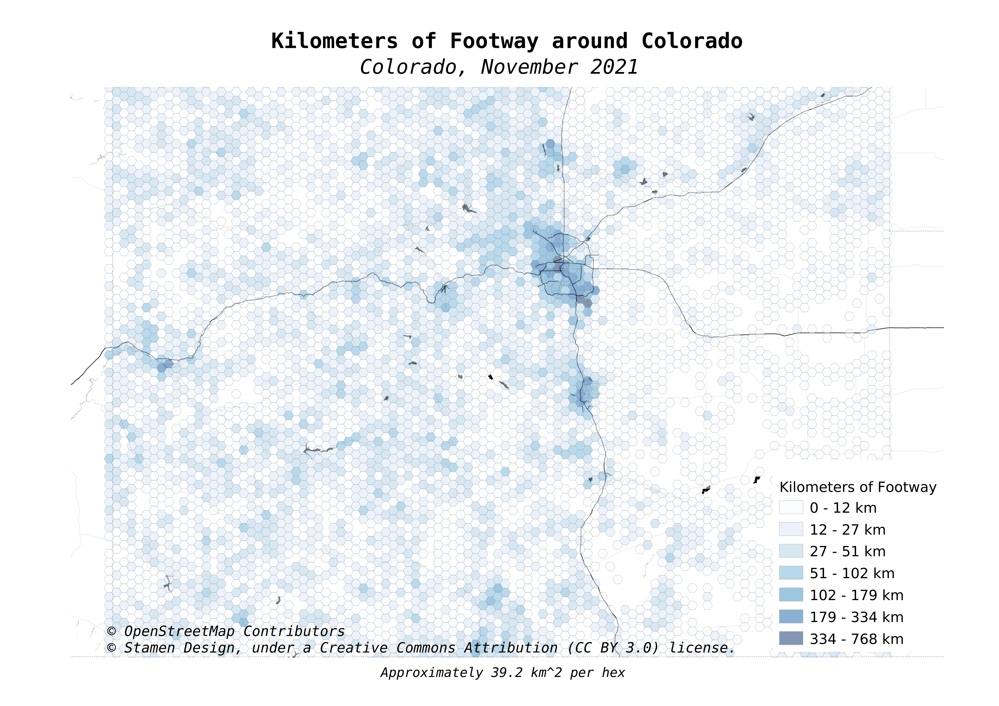
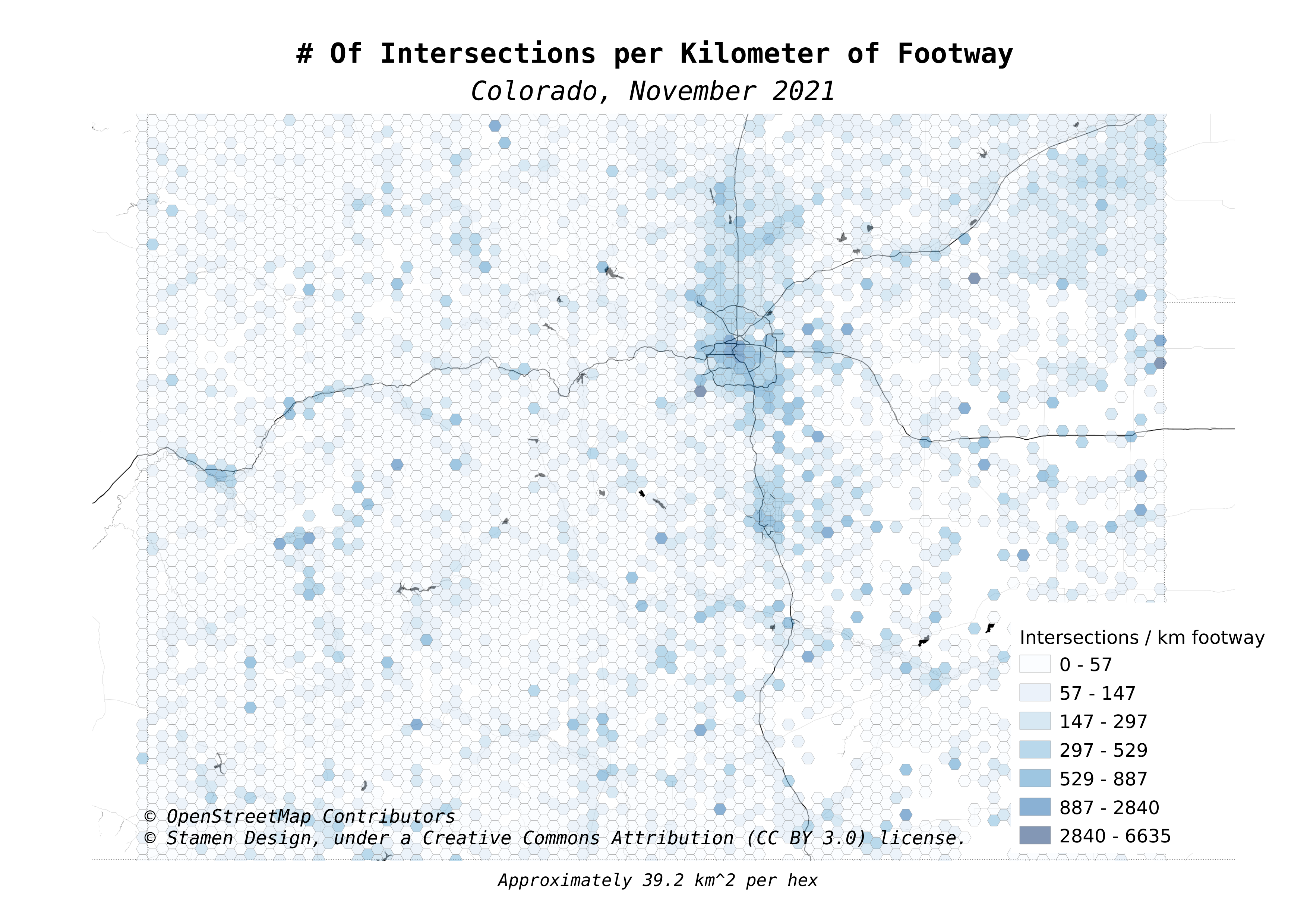
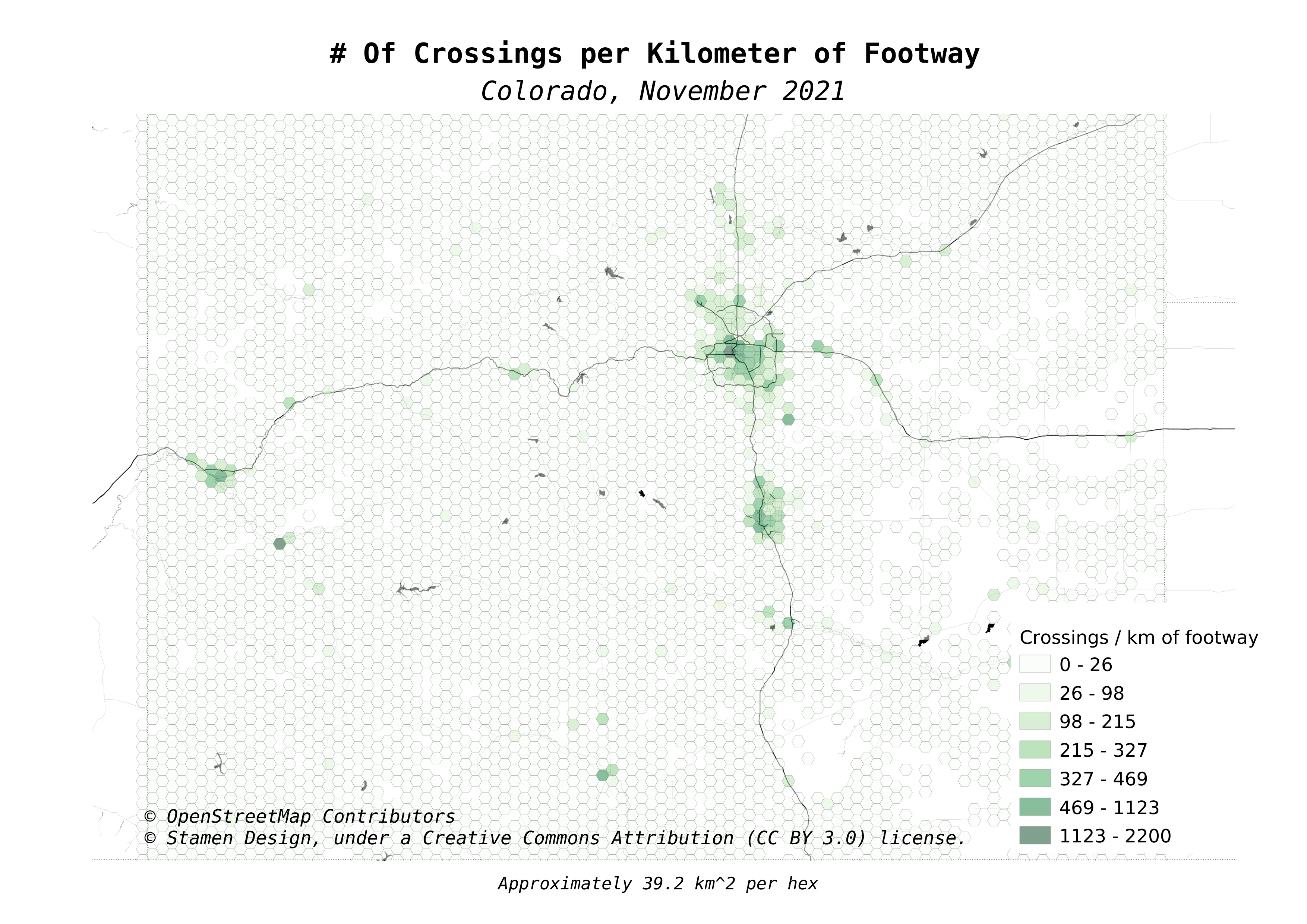
The map at the beginning of this post zoomed in to focus on the Denver metro region. The maps here look at the statewide data for Colorado.

First up is a map showing how prevalent footways are in various regions in the OpenStreetMap data. This shows how many kilometers of footway paths are in each hexagon.

The next map shows the count of intersections detected per kilometer of footway.

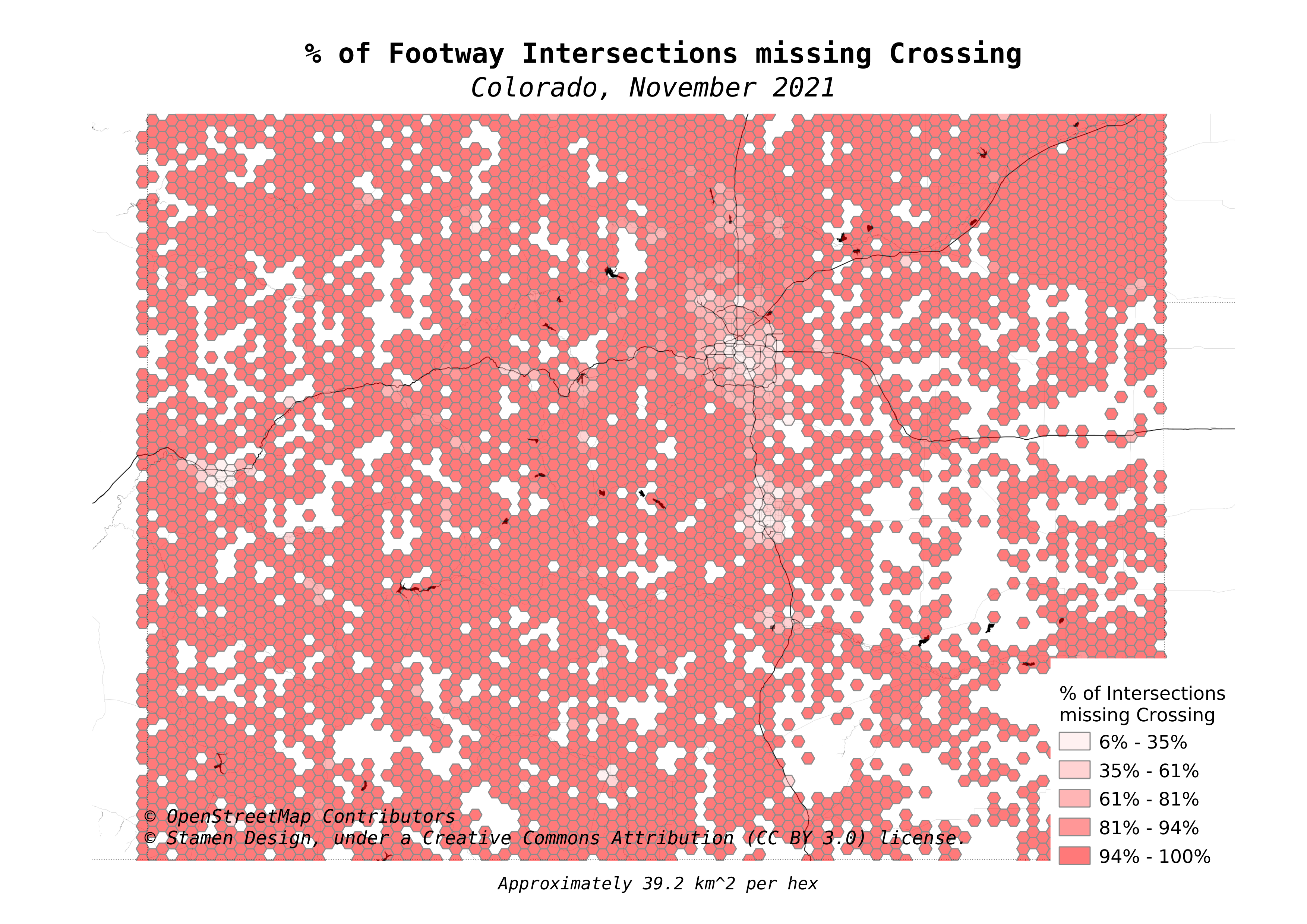
The following map changes the visualization from intersections to crossings. Comparing this map to the above map shows that in general, crossings are predominately found in the cities. Rural areas are largely vacant of crossing tags in the data.

The final map is the statewide view of the map at the top of the post. This is the calculated % of intersections between foot paths and motorized paths that are missing the crossing tag.

Summary

This post showed how I used a non-standard trick of expanding PostGIS lines out to the individual points that they are created from. This allowed for simple spatial joins between point layers to find intersections as defined by OpenStreetMap as sharing a node. Aggregating the details back to the roads, and ultimately up to hexagons enabled a visualization to highlight where crossings have and have not been marked in the data.

Need help with your PostgreSQL servers or databases? Contact us to start the conversation!