Timescale, Compression and OpenStreetMap Tags

This post captures my initial exploration with the Timescale DB extension in Postgres. I have watched Timescale with interest for quite some time but had not really experimented with it before now. I am considering Timescale as another solid option for improving my long-term storage of OpenStreetMap data snapshots. Naturally, I am using PostGIS enabled databases filled with OpenStreetMap data.

I started looking at restructuring our OpenStreetMap data with my post Why Partition OpenStreetMap data? That post has an overview of the historic use case I need to support. While my 1st attempt at declarative partitioning ran into a snag, my 2nd attempt worked rather well. This post looks beyond my initial requirements for the project and establishes additional benefits from adding Timescale into our databases.

Timescale benefits

There are two main reasons I am looking into Timescale as an option over Postgres' built-in declarative partitioning:

• No need to manually create partitions
• Compression is tempting

New partitions with Postgres' declarative partitioning must be created manually. The syntax isn't terribly tricky and the process can be automated, but it still exists therefore it still needs to be managed. When using Timescale's hypertables new partitions are handled behind the scenes without my direct intervention. The other temptation from Timescale is their columnar-style compression on row-based data. In standard Postgres, the only time compression kicks in is at the row level when a single row will exceed a specified size (default 2kb). See my post on large text data in Postgres that discusses compression in Postgres. Timescale has been writing about their compression so I figured it was time to give it a go. While compression wasn't one of the original goals I had outlined... it would be nice!!

Setup for testing

I installed Timescale 2.4.0 on an Ubuntu 20.04 instance following their instructions. I already had Postgres 13 and PostGIS 3.1 installed. After installing Timescale the postgresql.conf file needs to be updated to add timescaledb to shared_preload_libraries. I always have pg_stat_statements enabled, so my line in postgresql.conf looks like this:

shared_preload_libraries = 'pg_stat_statements,timescaledb'

Now the Timescale extension is ready to be created and used in our databases.

CREATE EXTENSION timescaledb;

The test database has five (5) schemas loaded with OpenStreetMap data for Colorado on different dates. The data was loaded to PostGIS using PgOSM Flex v0.2.1 and osm2pgsql v1.5.0. The total size of these OpenStreetMap data schemas is about 8.6 GB with the newest data (osm_co20210816) taking up 1,894 MB.

SELECT s_name, size_plus_indexes 
    FROM dd.schemas
    WHERE s_name LIKE 'osm%'
    ORDER BY s_name
;

┌────────────────┬───────────────────┐
│     s_name     │ size_plus_indexes │
╞════════════════╪═══════════════════╡
│ osm_co20181210 │ 1390 MB           │
│ osm_co20200816 │ 1797 MB           │
│ osm_co20210316 │ 1834 MB           │
│ osm_co20210718 │ 1884 MB           │
│ osm_co20210816 │ 1894 MB           │
└────────────────┴───────────────────┘

These snapshots from Colorado are taken my collection of PBF files I have accumulated over the years. The current size for Colorado loaded via PgOSM Flex is approaching 2GB. Ultimately, my plan is to take regular snapshots of the entire U.S. at least once a quarter. The current OpenStreetMap U.S. region loaded to PostGIS takes 67 GB and will likely reach 70 GB over the coming year. Loading this data using my previous scheme (no compression) will take nearly 300 GB on disk per year.

OpenStreetMap tags

Loading OpenStreetMap to PostGIS using PgOSM Flex creates a table named tags that stores each feature's key/value data in a JSONB column, also named tags. The tags data is a great starting point for me to get familiar with Timescale for two reasons:

• osm.tags is the largest table
• JSON data should compress nicely

I find it rather convenient that the best candidate for compression also happens to be a proportionally large table. To get an idea of the starting size of the tags table, the following query shows statistics for osm_co20210816.tags. This table contains almost 3.4 million rows and takes up 670 MB on disk, making this table responsible for 35% of the total size of the osm_co20210816 schema!

SELECT t_name, rows, size_plus_indexes, description
    FROM dd.tables
    WHERE s_name = 'osm_co20210816'
    ORDER BY size_bytes DESC
    LIMIT 1;

┌─[ RECORD 1 ]──────┬─────────────────────────────────────────────────────────┐
│ t_name            │ tags                                                    │
│ rows              │ 3,357,662
│ size_plus_indexes │ 681 MB                                                  │
│ description       │ OpenStreetMap tag data for all objects in source file. …│
│                   │… Key/value data stored in tags column in JSONB format.  │
└───────────────────┴─────────────────────────────────────────────────────────┘

An example of the data stored in the tags table.

SELECT *
    FROM osm_co20210816.tags
    WHERE osm_id = 709060219
        AND geom_type = 'W'
;

┌─[ RECORD 1 ]────────────────────────────────────────────────────────────────────────────┐
│ geom_type │ W                                                                           │
│ osm_id    │ 709060219                                                                   │
│ tags      │ {"gauge": "1435", "usage": "main", "railway": "rail", "voltage": "25000", "…│
│           │…frequency": "60", "electrified": "contact_line", "railway:track_ref": "4"}  │
│ osm_url   │ https://www.openstreetmap.org/way/709060219                                 │
└───────────┴─────────────────────────────────────────────────────────────────────────────┘

The tags data is helpful when the columns defined by PgOSM Flex in the main feature tables do not capture the need of your particular analysis.

Create hypertable

With the tags table identified as my starting point, it is time to test! I create a schema named osmts for my test playground.

CREATE SCHEMA osmts;
COMMENT ON SCHEMA osmts IS 'Objects for OpenStreetMap data in Timescale hypertables, possibly with compression.';

Create a new osmts.tags table based on one of the source tags tables. This uses Postgres' handy LIKE source_table syntax which allows me prepend the osm_date and region columns before the columns from the source table. Adding the non-standard columns to the beginning of the new table makes the INSERT statement in a few steps easier to write and maintain. The use of EXCLUDING INDEXES allows creating a new, more appropriate primary key for the hypertable.

CREATE TABLE osmts.tags
(
    osm_date DATE NOT NULL,
    region TEXT NOT NULL,
    LIKE osm_co20210816.tags EXCLUDING INDEXES
)
;
COMMENT ON TABLE osmts.tags IS 'Hypertable for historic OpenStreetMap tag data for all objects in source file. Key/value data stored in tags column in JSONB format.';

Use the create_hypertable() function to turn the osmts.tags table into a Timescale hypertable.

SELECT create_hypertable('osmts.tags', 'osm_date');
┌───────────────────┐
│ create_hypertable │
╞═══════════════════╡
│ (1,osmts,tags,t)  │
└───────────────────┘

The following query creates a new PRIMARY KEY that includes the osm_date and region into the scheme. I am intentionally putting osm_date last since it already has a dedicated index. The osm_id and geom_type columns will nearly always be used when querying the osmts.tags table so those are first. I don't have any data showing this is better for this use case (yet).

ALTER TABLE osmts.tags
    ADD CONSTRAINT pk_osmts_tags
    PRIMARY KEY (osm_id, geom_type, region, osm_date);

With the table created and prepared I begin to load data, starting with the oldest first. Hypertables are designed with the idea that newer data comes in later so testing in this order makes sense.

The following INSERT query moves data from the oldest tags table with a join to the matching pgosm_flex table to retrieve the osm_date and region.

INSERT INTO osmts.tags
SELECT p.osm_date, p.region, t.*
    FROM osm_co20181210.pgosm_flex p
    INNER JOIN osm_co20181210.tags t ON True
;
INSERT 0 2341324
Time: 12404.793 ms (00:12.405)

After the INSERT, run an ANALYZE to ensure Postgres and Timescale have updated statistics on the newly populated data.

ANALYZE osmts.tags;

A standard COUNT(*) confirms the row count from the previous INSERT.

SELECT COUNT(*) FROM osmts.tags;
┌─────────┐
│  count  │
╞═════════╡
│ 2341324 │
└─────────┘
(1 row)
Time: 268.845 ms

With Timescale's Hypertables there is a faster way to get a row count if exact numbers are not needed. The approximate_row_count() function runs significantly faster on large tables with results close to actual row counts. The difference from the prior result and the following result is only 1,620 different, a variance of 0.07% from the total.

SELECT approximate_row_count('osmts.tags');
┌───────────────────────┐
│ approximate_row_count │
╞═══════════════════════╡
│               2342944 │
└───────────────────────┘
(1 row)
Time: 56.806 ms

In this example, using approximate_row_count was 79% faster than COUNT(*) because it uses statistics instead of a full sequence scan. This is the same reason I often use our PgDD extension for row counts on regular Postgres tables.

Also of note, I had to run ANALYZE a couple times to get the approximate_row_count to be different from the actual row count... 😂

Compress hypertable

Timescale hypertables do not apply compression by default, it needs to be enabled. The following ALTER TABLE query defines how the table should be compressed. The Timescale docs on compression suggest that the segmentby columns should line up well with common WHERE clause patterns. The combination of segmentby columns and orderby columns are important to get right before you start doing this in production.

ALTER TABLE osmts.tags SET (
  timescaledb.compress,
  timescaledb.compress_segmentby = 'region, geom_type',
  timescaledb.compress_orderby = 'osm_id'
);

Note: The osm_date column is not included in the compression definition. That detail seems to be handled behind-the-scenes by Timescale.

Set a compression policy to automatically compress data older than a certain threshold. This is done with the add_compression_policy() function. The data loaded right now is from 2018, well beyond the 14 day threshold being set.

SELECT add_compression_policy('osmts.tags', INTERVAL '14 days');

After adding the policy, wait a minute or two for the compression to happen and check on the size using the results from the chunk_compression_stats() function. The results from the following query reports the data was 607 MB uncompressed and 45 MB when compressed.

Reduced size by 93%, not too shabby!

SELECT chunk_schema, chunk_name, compression_status,
        pg_size_pretty(before_compression_total_bytes) AS size_total_before,
        pg_size_pretty(after_compression_total_bytes) AS size_total_after
    FROM chunk_compression_stats('osmts.tags');

┌───────────────────────┬────────────────────┬────────────────────┬───────────────────┬──────────────────┐
│     chunk_schema      │     chunk_name     │ compression_status │ size_total_before │ size_total_after │
╞═══════════════════════╪════════════════════╪════════════════════╪═══════════════════╪══════════════════╡
│ _timescaledb_internal │ _hyper_28_33_chunk │ Compressed         │ 607 MB            │ 45 MB            │
└───────────────────────┴────────────────────┴────────────────────┴───────────────────┴──────────────────┘

Keep in mind, my goal is to implement this with the entire U.S., not just Colorado. The current size of the U.S. data is 67 GB with 27 GB of that bulk (40%!) in the tags table. Compressing this table by 93% should reduce each U.S. snapshot by around 25 GB.

Now that I have seen the compression working as advertised it is time to load the rest of the data from the remaining tags tables into osmts.tags.

INSERT INTO osmts.tags
SELECT p.osm_date, p.region, t.*
    FROM osm_co20200816.pgosm_flex p
    INNER JOIN osm_co20200816.tags t ON True
;

INSERT INTO osmts.tags
SELECT p.osm_date, p.region, t.*
    FROM osm_co20210316.pgosm_flex p
    INNER JOIN osm_co20210316.tags t ON True
;

INSERT INTO osmts.tags
SELECT p.osm_date, p.region, t.*
    FROM osm_co20210718.pgosm_flex p
    INNER JOIN osm_co20210718.tags t ON True
;

INSERT INTO osmts.tags
SELECT p.osm_date, p.region, t.*
    FROM osm_co20210816.pgosm_flex p
    INNER JOIN osm_co20210816.tags t ON True
;

Another ANALYZE and check the estimated row count, now reporting 15.3 million rows.

ANALYZE osmts.tags;
SELECT approximate_row_count('osmts.tags');

┌───────────────────────┐
│ approximate_row_count │
╞═══════════════════════╡
│              15356225 │
└───────────────────────┘

After a while, all but the newest data should end up compressed. If you are impatient like me you can manually compress the remaining chunks. The compression stats do not report the size of the uncompressed partition, but we can see that the four (4) compressed partitions now take up only 222 MB, down from a source size of 3,039 MB.

SELECT chunk_schema, chunk_name, compression_status,
        pg_size_pretty(before_compression_total_bytes) AS size_total_before,
        pg_size_pretty(after_compression_total_bytes) AS size_total_after
    FROM chunk_compression_stats('osmts.tags')
    ORDER BY chunk_name
;

┌───────────────────────┬────────────────────┬────────────────────┬───────────────────┬──────────────────┐
│     chunk_schema      │     chunk_name     │ compression_status │ size_total_before │ size_total_after │
╞═══════════════════════╪════════════════════╪════════════════════╪═══════════════════╪══════════════════╡
│ _timescaledb_internal │ _hyper_28_33_chunk │ Compressed         │ 607 MB            │ 45 MB            │
│ _timescaledb_internal │ _hyper_28_35_chunk │ Compressed         │ 790 MB            │ 57 MB            │
│ _timescaledb_internal │ _hyper_28_36_chunk │ Compressed         │ 810 MB            │ 59 MB            │
│ _timescaledb_internal │ _hyper_28_37_chunk │ Compressed         │ 832 MB            │ 61 MB            │
│ _timescaledb_internal │ _hyper_28_38_chunk │ Uncompressed       │ ¤                 │ ¤                │
└───────────────────────┴────────────────────┴────────────────────┴───────────────────┴──────────────────┘

We can use the hypertable_size() function to get the total size of the osmts.tags table, 1,057 MB, which allows use to calculate the size of the uncompressed chunk as 835 MB (1057 - 222).

SELECT pg_size_pretty(hypertable_size('osmts.tags'));

┌────────────────┐
│ pg_size_pretty │
╞════════════════╡
│ 1057 MB        │
└────────────────┘

Query performance

Each of the following queries was ran multiple times with EXPLAIN (ANALYZE) with a single representative timing picked to show here. The full plans are not shown, only the timings.

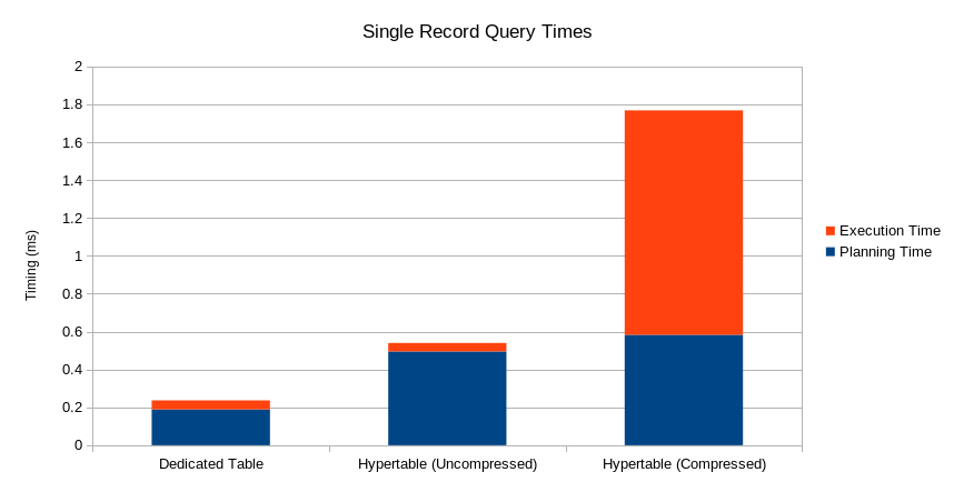
To check how this setup affects query performance I start by querying for a single record from the latest data in its original form. This is the baseline.

EXPLAIN (ANALYZE)
SELECT *
    FROM osm_co20210816.tags
    WHERE osm_id = 709060219
        AND geom_type = 'W'
;

Planning Time: 0.189 ms
Execution Time: 0.048 ms

Now query for the same record from the same date, just using the osmts.tags table. The updated query requires an additional filter on osm_date the previous query did not need. The planning now takes nearly 0.5 ms but the planning plus execution time is still under 1ms total. This date's data is the portion that is not compressed.

EXPLAIN (ANALYZE)
SELECT *
    FROM osmts.tags
    WHERE osm_id = 709060219
        AND geom_type = 'W'
        AND osm_date = '2021-08-16'
;

Planning Time: 0.495 ms
Execution Time: 0.045 ms

Now a query to see how query performance changes when pulling the same record from one of the historic, compressed partitions. The execution time is now a little more than 1 ms.

EXPLAIN (ANALYZE)
SELECT *
    FROM osmts.tags
    WHERE osm_id = 709060219
        AND geom_type = 'W'
        AND osm_date = '2020-08-16'
;

Planning Time: 0.583 ms
Execution Time: 1.185 ms

Not slow by any means, but this timing makes it apparent the overhead from compression isn't free either.

Summary

This post has started exploring Timescale hypertables and compression by loading in five snapshots of unstructured OpenStreetMap key/value tags data. Creating the hypertable and enabling compression went smoothly. The compression ratio (93%) was inline with Timescale's advertised expectations and query performance appears to be more than satisfactory for my typical use case.

While my initial success here is exciting, this is only part of the journey. The tags data is only one OpenStreetMap table loaded by PgOSM Flex. I have plans to keep roads, waterways, places and a few other key tables over time as well. These other tables all contain PostGIS data and will not compress as nicely as the tags. Initial testing shows the tables with PostGIS data are achieving 40-45% compression instead of > 90% achieved here. It also comes with a caveat, but this post has grown long enough already.

Stay tuned for more details on using Timescale's compression with PostGIS data.

Need help with your PostgreSQL servers or databases? Contact us to start the conversation!