
First Review of Partitioning OpenStreetMap
My previous two posts set the stage to evaluate declarative Postgres partitioning for OpenStreetMap data. This post outlines what I found when I tested my plan and outlines my next steps. The goal with this series is to determine if partitioning is a path worth going down, or if the additional complexity outweighs any benefits. The first post on partitioning outlined my use case and why I thought partitioning would be a potential benefit. The maintenance aspects of partitioning are my #1 hope for improvement, with easy and fast loading and removal of entire data sets being a big deal for me.
The second post detailed my approach to partitioning to allow me to partition based on date and region. In that post I even bragged that a clever workaround was a suitable solution.
"No big deal, creating the
osmp.pgosm_flex_partitiontable gives eachosm_date+regiona single ID to use to define list partitions." -- Arrogant MeRead on to see where that assumption fell apart and my planned next steps.
I was hoping to have made a "Go / No-Go" decision by this point... I am currently at a solid "Probably!"
Load data
For testing I simulated Colorado data being loaded once per month on the 1st of each month and North America once per year on January 1. This was conceptually easier to implement and test than trying to capture exactly what I described in my initial post. This approach resulted in 17 snapshots of OpenStreetMap being loaded, 15 with Colorado and two with North America. I loaded this data twice, once using the planned partitioned setup and the other using a simple stacked table to compare performance against.
The parent partitioned objects live in the osmp schema with the actual data living
in schemas named osm_1, osm_2, etc. The numbers in the schema line up with
the partition key as a side effect of scripting out the import.
The stacked data lives in a table with the same structure in the osms schema.
The partition lookup table can show us what we're working with.
SELECT *
    FROM osmp.pgosm_flex_partition
;
The id values shown here have a couple gaps (missing 2, 16 and 18).
I made mistakes during testing that burned those IDs via the IDENTITY.
┌────┬────────────┬────────────────────────────┐
│ id │  osm_date  │           region           │
╞════╪════════════╪════════════════════════════╡
│  1 │ 2020-01-01 │ north-america/us--colorado │
│  3 │ 2020-02-01 │ north-america/us--colorado │
│  4 │ 2020-03-01 │ north-america/us--colorado │
│ .. │ .......... │ .......................... │
│ 15 │ 2021-02-01 │ north-america/us--colorado │
│ 16 │ 2021-02-18 │ north-america/us--colorado │
│ 17 │ 2021-01-01 │ north-america              │
│ 19 │ 2020-01-01 │ north-america              │
└────┴────────────┴────────────────────────────┘
Partitioned versus Stacked
Both the stacked table and the partitioned table report a total of nearly 92 million rows. This verifies I did get the same data loaded to both tables. While 92 M rows is not giant sized data, and may not fully illustrate the full benefits from partitioning, it is large enough to put my initial expectations to the test.
SELECT 'stacked' AS src, COUNT(*) FROM osms.road_line
UNION
SELECT 'partitioned' AS src, COUNT(*) FROM osmp.road_line;

┌─────────────┬──────────┐
│     src     │  count   │
╞═════════════╪══════════╡
│ partitioned │ 91826226 │
│ stacked     │ 91826226 │
└─────────────┴──────────┘
A key benefit of partitioned data are the index sizes for each partition should be
considerably smaller than the index sizes of the stacked data.
The following query uses the pg_catalog.pg_stat_all_indexes system catalog to
find the indexes in the various road_line tables.
SELECT ai.schemaname AS s_name, ai.relname AS t_name,
        ai.indexrelname AS index_name,
        pg_size_pretty(pg_relation_size(quote_ident(ai.schemaname)::text || '.' || quote_ident(ai.indexrelname)::text)) AS index_size,
        pg_relation_size(quote_ident(ai.schemaname)::text || '.' || quote_ident(ai.indexrelname)::text) AS index_size_bytes
    FROM pg_catalog.pg_stat_all_indexes ai
    WHERE ai.schemaname LIKE 'osm%'
        AND ai.relname = 'road_line'
    ORDER BY index_size_bytes DESC
    LIMIT 10
;

┌────────┬───────────┬──────────────────────────────────────┬────────────┬──────────────────┐
│ s_name │  t_name   │              index_name              │ index_size │ index_size_bytes │
╞════════╪═══════════╪══════════════════════════════════════╪════════════╪══════════════════╡
│ osms   │ road_line │ gix_osms_road_line                   │ 5080 MB    │       5326880768 │
│ osms   │ road_line │ pk_osm_road_line_osm_id              │ 3823 MB    │       4008542208 │
│ osm_17 │ road_line │ road_line_geom_idx                   │ 2116 MB    │       2219122688 │
│ osm_19 │ road_line │ road_line_geom_idx                   │ 2005 MB    │       2102788096 │
│ osm_19 │ road_line │ pk_osm_road_line_partition_id_osm_id │ 1198 MB    │       1255743488 │
│ osm_17 │ road_line │ pk_osm_road_line_partition_id_osm_id │ 1198 MB    │       1255743488 │
│ osm_17 │ road_line │ ix_osm_road_line_highway             │ 265 MB     │        277889024 │
│ osm_19 │ road_line │ ix_osm_road_line_highway             │ 265 MB     │        277889024 │
│ osm_5  │ road_line │ road_line_geom_idx                   │ 91 MB      │         95600640 │
│ osm_4  │ road_line │ road_line_geom_idx                   │ 91 MB      │         95387648 │
└────────┴───────────┴──────────────────────────────────────┴────────────┴──────────────────┘
This query also came in handy when I was reviewing improvements from the BTree deduplication in Postgres 13.
The two largest indexes are the indexes on the simple stacked
table, osms.road_line.
Its GIST index is 5GB and the primary key is nearly 4GB.
As more data is loaded these indexes will continue to grow. This becomes a
performance problem when your indexes
no longer fit nicely in RAM and have to be read from disk.
The GIST indexes on the two North America partitions
(osm_17) and (osm_19) are the next two largest indexes, at roughly 2GB each.
Those are shortly followed by the two PKs on those N.A. tables at 1.2 GB each.
The next largest index sizes drop down to the Colorado data sets (osm_5 and osm_4)
the indexes get nice and compact, indicating the size difference between Colorado vs. North America.
As more data is added, each partitioned index stays representative to the size
of that batch of data.
The size of these indexes matters because when partition pruning occurs, Postgres only has to use the indexes from some of the partitions. Searching a smaller index will be faster than searching a larger index, and it is more likely a smaller index will fit inside (and stay inside) RAM. This improvement can be seen below.
Querying
To test my expectations out I tried a number of different queries between the partitioned data and stacked data to compare plans and performance. It was in this stage that I ran into a snag that I mentioned at the beginning. The queries here illustrate the problem I ran into.
Each query below returns these two rows, providing a simple row count for the selected two sets of data
┌────────────────────────────┬────────────┬────────┐
│           region           │  osm_date  │ count  │
╞════════════════════════════╪════════════╪════════╡
│ north-america/us--colorado │ 2020-01-01 │ 813696 │
│ north-america/us--colorado │ 2021-01-01 │ 813696 │
└────────────────────────────┴────────────┴────────┘
The row counts are identical for the two different dates because I loaded the same OSM data over and over for testing. That should not have any impact to the queries tested here.
Query 1
The first version of the query uses the partitioned table. It joins to the
osmp.pgosm_flex_partition table allow displaying the friendly region and osm_date
seen above, but the actual filtering is done on those IDs (1, 14) instead of
the friendly name and description.
EXPLAIN (ANALYZE, BUFFERS, VERBOSE, SETTINGS)
SELECT p.region, p.osm_date, COUNT(*)
    FROM osmp.road_line r
    INNER JOIN osmp.pgosm_flex_partition p
        ON r.pgosm_flex_partition_id = p.id
    WHERE r.pgosm_flex_partition_id IN (1, 14)
    GROUP BY p.region, p.osm_date
;
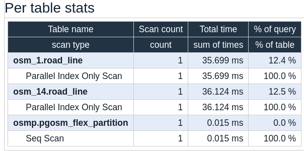
This query runs in 288 ms, pretty good performance for a COUNT(*) query on a
big(-ish) table. The query plan
shows that the Postgres planner was able to prune out unnecessary partitions before
execution started. The plan does not explicitly tell us that, we can infer
pruning occurred because only the osm_1 and osm_14 tables were accessed via their indexes, each taking about 36 ms.
Query 2
The first query shows partition pruning working as I would expect but I do not want to write queries using the IDs. I've tried using systems like that before, not even people that love writing code want to do that regularly.
Instead, I want to write queries like the following example to be clear at exactly what data is being used. Remember, my use case is predominantly analytical queries so having obvious, transparent code is a good thing. The following query is clear about what data is being included.
EXPLAIN (ANALYZE, BUFFERS, VERBOSE, SETTINGS)
SELECT p.region, p.osm_date, COUNT(*)
    FROM osmp.road_line r
    INNER JOIN osmp.pgosm_flex_partition p
        ON r.pgosm_flex_partition_id = p.id
            AND p.osm_date IN ('2021-01-01', '2020-01-01')
            AND p.region = 'north-america/us--colorado'
    GROUP BY p.region, p.osm_date
;
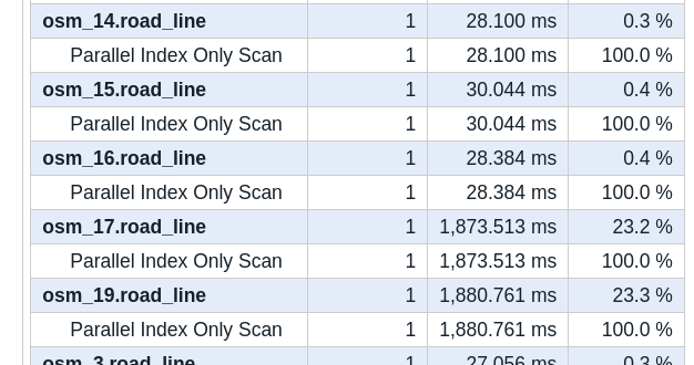
Unfortunately, this query takes more than 8 seconds to complete! A look at
the Per table stats from the associated query plan
shows that Postgres did not prune partitions for this query, instead decides
to scan every partition's index.
The following screenshot is a snippet of that table, showing the index scans
covering the two North America partitions (osm_17 and osm_19) each took
close to 2 seconds!
I tried rewriting the above query a number of different ways to try to get Postgres to prune partitions like it did in Query 1. I used sub-queries, CTEs,
EXISTS, etc. but was unable to find a solution that would get Postgres to prune partitions without hard-coding IDs.
Query 3
The two queries above have illustrated that queries on partitioned data can be:
- fast when partition pruning kicks in
- slow when partition pruning does not kick in
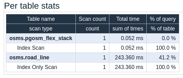
How does this compare to the stacked method? This 3rd query uses the improved (human friendly) join from Query 2, but now queries the stacked table instead of the partitioned table.
EXPLAIN (ANALYZE, BUFFERS, VERBOSE, SETTINGS)
SELECT s.region, s.osm_date, COUNT(*)
    FROM osms.pgosm_flex_stack s
    INNER JOIN osms.road_line r
        ON r.pgosm_flex_stack_id = s.id
            AND s.osm_date IN ('2021-01-01', '2020-01-01')
            AND s.region = 'north-america/us--colorado'
    GROUP BY s.region, s.osm_date
;
This query on the stacked table returns results with pretty good performance (591 ms). That is far better than the 8 seconds from Query 2, but it still takes twice as long as Query 1 when partition pruning was used. Scanning the index on the stacked table took 243 ms, while the two small index scans on the partitioned table took a total of 70 ms. This helps highlight that there are real benefits when partitioning works as desired, scanning smaller indexes is always going to be faster than scanning larger indexes!
Revisit requirements
Query 2 is an example of the type of query I thought I wanted to write.
The structure I had settled on to get to this point was determined by using
a lot of "The way I've always done it" plus
the documented details
for Postgres' partitioning. I had expected partition pruning to work via
JOIN conditions even though the documentation does not explicitly state it should work.
It doesn't seem unreasonable to expect, but also doesn't seem to work (at least yet!).
The reality is my original requirements are not going to provide the
benefit I want, though I still think
I can get the benefits I want from Postgres' partitioning.
Knowing my original requirements of having both date and region represented in the partition key
are holding me back, I reconsidered
why I wanted to partition on both osm_date and region.
Yes, I need to be able to track the region that was loaded, but that detail
has no relevance to the partitioning of the data! If I load North America today,
I do not also need to load Colorado additionally.
The osm_date is the only part that needs to be in the partition key, and that
means I can put it directly in the table instead of an ID.
OpenStreetMap data loaded via PgOSM-Flex gets loaded with meta information automatically tracked for us in the
pgosm_flextable of each schema. This query shows some of the meta-data included for theosm_19schema.SELECT osm_date, region, pgosm_flex_version, osm2pgsql_version FROM osm_19.pgosm_flex; ┌────────────┬───────────────┬────────────────────┬───────────────────┐ │ osm_date │ region │ pgosm_flex_version │ osm2pgsql_version │ ╞════════════╪═══════════════╪════════════════════╪═══════════════════╡ │ 2020-01-01 │ north-america │ 0.1.1-f488d7b │ 1.4.1 │ └────────────┴───────────────┴────────────────────┴───────────────────┘
The date is the important part. The region detail is still available in the meta-information. With this in mind, I will restructure and simplify the partitioning scheme and give this another go. Stay tuned for that post!
Version and Hardware
Postgres 13.2 was used for this post on a memory optimized Digital Ocean droplet with 8 CPU, 64 GB RAM and 600 GB SSD.
SELECT version();

┌──────────────────────────────────────────────────────────────────────────────────────────────────┐
│                                             version                                              │
╞══════════════════════════════════════════════════════════════════════════════════════════════════╡
│ PostgreSQL 13.2 (Ubuntu 13.2-1.pgdg20.04+1) on x86_64-pc-linux-gnu, compiled by gcc (Ubuntu 9.3.…│
│…0-17ubuntu1~20.04) 9.3.0, 64-bit                                                                 │
└──────────────────────────────────────────────────────────────────────────────────────────────────┘
Summary
This post covered what I found from my initial tests implementing my plan to partition OpenStreetMap data in our Postgres databases. This attempt was not the final solution as hoped, but was productive and shows definite promise. I will adjust a little bit of code, run tests again and hopefully the next post can focus on the long term maintenance benefits associated with this change.
Need help with your PostgreSQL servers or databases? Contact us to start the conversation!
 Mastodon