
PostGIS: Tame your spatial data (Part 2)
In a previous post PostGIS: Tame your spatial data
I illustrated how large-area polygons in your spatial data can take up a lot of space.
That post examined one method (ST_Simplify) to reduce the size of the data (45% reduction of size on disk)
in order to improve performance (37% faster queries).
The goal of reductions like this are to improve the life of the analysts
working with spatial data for their job.
These analysts are often using spatial data within a GIS tool such as QGIS, and in
those tools Time-to-Render (TTR) is quite important.
The topic of that prior post solved a specific problem (large polygons), and unfortunately that solution can't be applied to all problems related to the size of spatial data.
This post is an advanced topic of the series PostgreSQL: From Idea to Database.
Set the stage
This post uses PostgreSQL 11 and PostGIS 2.5 running on a dual-core Ubuntu 18 VM within VirtualBox.
The table (osm.roads_line) contains a large set of lines (nearly 500k) from
OpenStreetMap (OSM) including everything from major
interstate highways (e.g. I-70, I-25) to individual sidewalks throughout Colorado.
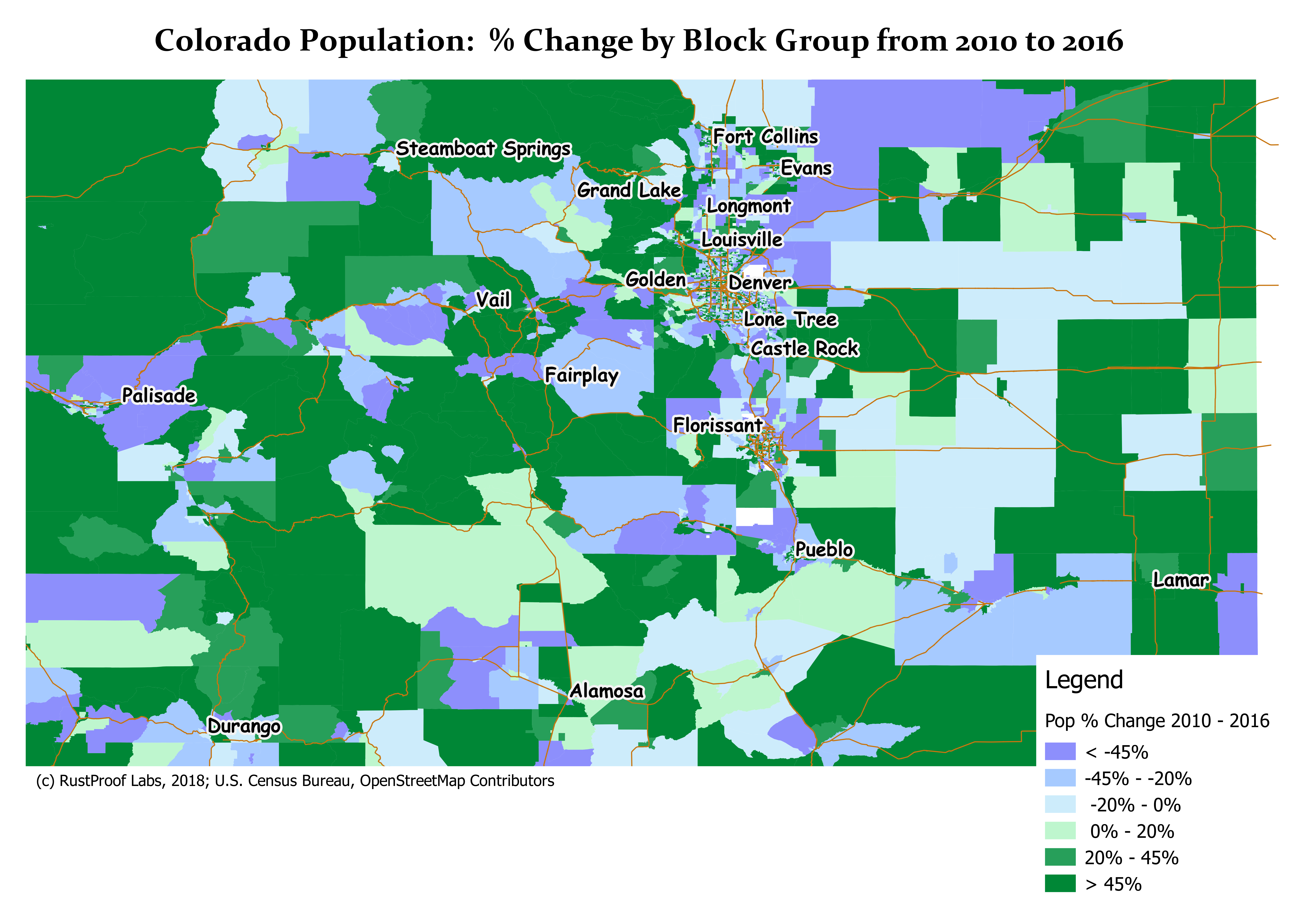
Let's use a scenario where I need to generate a map visualizing the entire state of Colorado, or ats least a large portion of it. An example of this are the maps I generated for Visualizing Colorado's Growing Population: 2010 to 2016. Notice that each of the maps in that post show the major road networks around Colorado.
The following query shows more details about the contents of the data within osm.roads_line.
SELECT 'original' AS src, COUNT(*) AS row_count,
        MIN(ST_NPoints(way)) AS min_points,
        MAX(ST_NPoints(way)) AS max_points,
        ROUND(AVG(ST_NPoints(way)), 2) AS avg_points,
        SUM(ST_NPoints(way)) AS total_points,
        SUM(ST_MemSize(way)) / 1024 AS total_geom_size_kb
    FROM osm.roads_line;
┌───────────┬───────────┬────────────┬────────────┬────────────┬──────────────┬────────────────────┐
│    src    │ row_count │ min_points │ max_points │ avg_points │ total_points │ total_geom_size_kb │
╞═══════════╪═══════════╪════════════╪════════════╪════════════╪══════════════╪════════════════════╡
│ original  │    459694 │          2 │       1959 │      14.06 │      6462469 │             113877 │
└───────────┴───────────┴────────────┴────────────┴────────────┴──────────────┴────────────────────┘
See
ST_NPointsandST_MemSizefor more information about the PostGIS functions used in the above query.
Many small objects
In this case, ST_Simplify won't provide any benefit. The goal of ST_Simplify
is to make complex objects less complex, by reducing the number of points.
My prior example was
used on data with more than 700 points per row, while this table has only 14 points
per row. In this example, the real problem is the number of rows being pushed from
PostgreSQL/PostGIS to QGIS for the visualization.
The roads visualized on the above thematic map uses a total of 15,778 rows, or 3.4% of the total rows
from the osm.roads_line table.
If you're a database professional, you may be thinking that this sounds like a
nice, selective index
that can be created and no big deal. Right? Sorry, it doesn't work like that in
GIS-analyst land.
Row count matters
Given a database of spatial data, a GIS analyst using QGIS will connect to the database,
and proceed to drag a roads "layer" into their project. I know, because that's what I do
when I'm wearing my analyst hat.
So what happens when we drag and drop a table with half a million rows?
Luckily for me, I have pg_stat_statements
installed so I can see what is going on within PostgreSQL.
To see the queries running when I work in QGIS, I simply run
SELECT pg_stat_statements_reset(); before QGIS queries any data and see what comes
through the pg_stat_statements.
One query that caught my attention immediately was this cursor declaration:
DECLARE qgis_1 BINARY CURSOR FOR
    SELECT st_asbinary("way",'NDR'),ctid,"code"::text,"highway"::text
        FROM "osm"."roads_line"
        WHERE "way"
            && st_makeenvelope(-12161779.75917431153357029,4328013.5903669772669673,-11263246.45917431451380253,5119382.36834862548857927,900913);
Seeing that the cursor is named qgis_1 made me suspicious there is more than
one query going on. The following query showed that I was right, but the number
of cursors itself isn't the actual problem here (never thought I would say that!).
The real problem is that the qgis_1 cursor was accessed 231 times!
If you just look at the database stats, the total time for execution against qgis_1
was only 1.5 seconds. That puts the average execution time quite low (15ms so what is
the problem??
That only represents the time the database spent working. Network latency sucks, and the timing shown by the database does not represent the time the analyst spends waiting for QGIS to actually render something useful.
SELECT query, calls, total_time
        FROM pg_stat_statements
        WHERE query LIKE 'FETCH FORWARD % FROM qgis%'
        ORDER BY calls DESC
        ;
┌────────────────────────────────┬───────┬─────────────┐
│             query              │ calls │ total_time  │
╞════════════════════════════════╪═══════╪═════════════╡
│ FETCH FORWARD 2000 FROM qgis_1 │   231 │ 1509.337915 │
│ FETCH FORWARD 2000 FROM qgis_2 │     2 │   22.718511 │
│ FETCH FORWARD 2000 FROM qgis_3 │     2 │    38.52645 │
│ FETCH FORWARD 2000 FROM qgis_9 │     1 │   23.889876 │
│ FETCH FORWARD 2000 FROM qgis_5 │     1 │    3.105468 │
│ FETCH FORWARD 2000 FROM qgis_8 │     1 │    5.296408 │
│ FETCH FORWARD 2000 FROM qgis_4 │     1 │    7.149537 │
│ FETCH FORWARD 2000 FROM qgis_6 │     1 │   24.612578 │
│ FETCH FORWARD 2000 FROM qgis_7 │     1 │    2.213806 │
└────────────────────────────────┴───────┴─────────────┘
(9 rows)
Once again, it is not the database at fault for slow performance!
Network traffic
The network traffic generated by this QGIS loading this data tells another story. Windows' Task Manager shows that to download and render the OSM road data, there's nearly a full minute showing more than a dozen large bursts of network traffic.
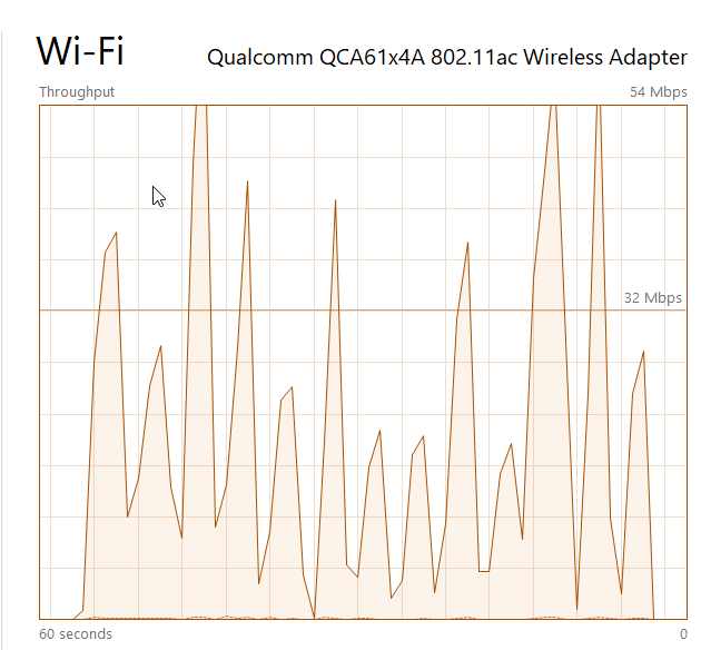
Remember above where it showed the qgis_1 cursor was fetched from 231 times?
I haven't looked at the source code for QGIS, so this next bit is pure conjecture....
Each of those large bursts across the network represents QGIS running the
FETCH FORWARD 2000... queries, and the valleys are where it is pausing.
I would have to guess that QGIS fetches data from PostgreSQL 15-20 times
as quickly as possible (causing the spikes)
followed by a delay in querying (to be nice) in the range of 2-5 seconds (causing the valleys).
What are all these rows?
Think of a major highway in your area. For example, if you live anywhere near Denver, Colorado you most likely know about I-70. Querying our table for the rows that represent I-70 across Colorado returns 1,647 rows of data with a total of 19,281 nodes (points).
SELECT COUNT(*) AS row_count,
        MIN(ST_NPoints(way)) AS min_points,
        MAX(ST_NPoints(way)) AS max_points,
        ROUND(AVG(ST_NPoints(way)), 2) AS avg_points,
        SUM(ST_NPoints(way)) AS total_points,
        SUM(ST_MemSize(way)) / 1024 AS total_geom_size_kb
 FROM osm.roads_line
  WHERE ref ILIKE '%I 70%'
;
┌───────────┬────────────┬────────────┬────────────┬──────────────┬────────────────────┐
│ row_count │ min_points │ max_points │ avg_points │ total_points │ total_geom_size_kb │
╞═══════════╪════════════╪════════════╪════════════╪══════════════╪════════════════════╡
│      1647 │          2 │        217 │      11.71 │        19281 │                342 │
└───────────┴────────────┴────────────┴────────────┴──────────────┴────────────────────┘
Goal: Reduce row count
Knowing that 2,000 rows is the apparent max per batch from the database is helpful and
gives us a starting point for optimization. In the past, I have always used
PostGIS's ST_Union()
to aggregate spatial data but have
recently been using ST_Collect() instead.
ST_Collect is faster, and operates in the way I typically assumed ST_Union worked
anyway.
Smaller tests showed
ST_Collectrunning at least 80% faster thanST_Union. Larger tests showed 98+% increases by usingST_Collect.
Before we get into those spatial aggreations...
Filter results
When creating a thematic layer, the first thing to consider are ways to reduce
the row count in the WHERE clause.
This is a general best-practice of databases, but is worth discussing.
Thematic GIS layers (tables) should only include rows that will be viewed when
zoomed way out. When thinking about thematic layers for the state level, there
is no need to consider all the sidewalks, residential roads, or parking lots.
Enter, the WHERE clause:
WHERE highway IN ('motorway','motorway_link','primary','primary_link',
            'secondary','secondary_link','tertiary','trunk','trunk_link')
By adding that filter to the osm.roads_line table it reduces the rows returned
to 47,413, 10% of the total rows.
In QGIS this would mean only 25 queries
need to be ran (down from 231). While that's a great reduction, 25 queries to load
a single layer seems like a lot to me. What if there's a 100ms latency in
the network?
100 ms * 25 queries = 2500 ms = 2.5 seconds
Even a relatively small latency in the network can introduce quite large, disruptive delays to the analysts.
Aggregate with ST_Collect()
The ST_Collect() function in
PostGIS aggregates spatial data, much like the
SUM() function aggregates numbers by adding them up.
By combining the smartly designed filter above with some spatial aggregation,
our data is about ready for thematic use.
CREATE TABLE osm.roads_line_hwy_ref_collect AS
SELECT name, ref, highway, code, ST_Collect(way) AS way
    FROM osm.roads_line
    WHERE highway IN ('motorway','motorway_link','primary','primary_link',
                'secondary','secondary_link','tertiary','trunk','trunk_link')
    GROUP BY name, highway, ref, code;
SELECT 5853
Time: 504.445 ms
Don't forget to create a GIST index on your spatial columns!
CREATE INDEX GIX_osm_roads_line_hwy_ref_collect
    ON osm.roads_line_hwy_ref_collect
    USING GIST (way);
Assess our reduction
Now to compare the original osm.roads_line table with the table created using
ST_COllect().
At 5,853 rows, that should only require 4 queries from QGIS (instead of 25, or 231).
You'll notice the number of points per row has increased dramatically, but still
far below where it becomes a problem.
SELECT 'original' AS src, COUNT(*) AS row_count,
        MIN(ST_NPoints(way)) AS min_points,
        MAX(ST_NPoints(way)) AS max_points,
        ROUND(AVG(ST_NPoints(way)), 2) AS avg_points,
        SUM(ST_NPoints(way)) AS total_points,
        SUM(ST_MemSize(way)) / 1024 AS total_geom_size_kb
    FROM osm.roads_line
UNION
SELECT 'ST_Collect()' AS src, COUNT(*) AS row_count,
        MIN(ST_NPoints(way)) AS min_points,
        MAX(ST_NPoints(way)) AS max_points,
        ROUND(AVG(ST_NPoints(way)), 2) AS avg_points,
        SUM(ST_NPoints(way)) AS total_points,
        SUM(ST_MemSize(way)) / 1024 AS total_geom_size_kb
    FROM osm.roads_line_hwy_ref_collect;
┌──────────────┬───────────┬────────────┬────────────┬────────────┬──────────────┬────────────────────┐
│     src      │ row_count │ min_points │ max_points │ avg_points │ total_points │ total_geom_size_kb │
╞══════════════╪═══════════╪════════════╪════════════╪════════════╪══════════════╪════════════════════╡
│ original     │    459694 │          2 │       1959 │      14.06 │      6462469 │             113877 │
│ ST_Collect() │      5853 │          2 │      29414 │     107.77 │       630794 │              10406 │
└──────────────┴───────────┴────────────┴────────────┴────────────┴──────────────┴────────────────────┘
Revisiting I-70
Earlier, I showed that the full OSM road data set uses 1,647 rows of data to represent the
expanse of I-70 across Colorado.
The following query compares the original I-70 data to the version created from
ST_Collect().
The reduced version is only 70 rows of data.
SELECT 'original' AS src,
        COUNT(*) AS row_count,
        MIN(ST_NPoints(way)) AS min_points,
        MAX(ST_NPoints(way)) AS max_points,
        ROUND(AVG(ST_NPoints(way)), 2) AS avg_points,
        SUM(ST_NPoints(way)) AS total_points,
        SUM(ST_MemSize(way)) / 1024 AS total_geom_size_kb
 FROM osm.roads_line
  WHERE ref ILIKE '%I 70%'
UNION
SELECT 'ST_Collect()' AS src,
        COUNT(*) AS row_count,
        MIN(ST_NPoints(way)) AS min_points,
        MAX(ST_NPoints(way)) AS max_points,
        ROUND(AVG(ST_NPoints(way)), 2) AS avg_points,
        SUM(ST_NPoints(way)) AS total_points,
        SUM(ST_MemSize(way)) / 1024 AS total_geom_size_kb
 FROM osm.roads_line_hwy_ref_collect
  WHERE ref ILIKE '%I 70%'
;

┌──────────────┬───────────┬────────────┬────────────┬────────────┬──────────────┬────────────────────┐
│     src      │ row_count │ min_points │ max_points │ avg_points │ total_points │ total_geom_size_kb │
╞══════════════╪═══════════╪════════════╪════════════╪════════════╪══════════════╪════════════════════╡
│ original     │      1647 │          2 │        217 │      11.71 │        19281 │                342 │
│ ST_Collect() │        70 │          2 │       4604 │     275.44 │        19281 │                316 │
└──────────────┴───────────┴────────────┴────────────┴────────────┴──────────────┴────────────────────┘
Materialized View
Reductions like this are a fantastic use of PostgreSQL's materialized views.
The following is more representative of what I use in our real environments.
In our osm databases, the _t suffix indicates it's a thematic layer.
CREATE MATERIALIZED VIEW osm.roads_line_t AS
SELECT name, ref, highway, code, ST_Collect(way) AS way
    FROM osm.roads_line
    WHERE highway IN ('motorway','motorway_link','primary','primary_link',
                'secondary','secondary_link','tertiary','trunk','trunk_link')
    GROUP BY name, highway, ref, code;
A thematic layer indicates data reduction has occurred, giving an indication of what to expect with data quality. Any time data is simplified (spatial, or not) meaning and precision is lost.
Materialized views allow us to create indexes on them too.
CREATE INDEX GIX_osm_roads_line_t_mv
    ON osm.roads_line_t
    USING GIST (way);
What about the analysts?
Ok, so what does all this mean to the end user in QGIS? Well, look at this 60-second view of what happens when QGIS loads the full data set from my local network.
Timings in QGIS
The following timings were taken 3 times for each query, measured manually based on time to render (TTR) in QGIS.
| Source | Time (s) | Reduction in TTR |
|---|---|---|
| Original | 50 | 0% |
| Original w/ Filter | 8 | -84% |
| ST_Collect() (table or mat. view) | 2.5 | -95% |
Summary
Spatial data in PostGIS is still data in the world's most advanced open source relational database, PostgreSQL. The same techniques we know for more traditional data hold true with spatial data in PostGIS. We simply(?) need to take the time to invest in learning the appropriate tools and techniques.
Need help with your PostgreSQL servers or databases? Contact us to start the conversation!
 Mastodon