
PostGIS: Tame your spatial data (Part 1)
The goal of this post is to examine and fix one common headache when using spatial data: its size. Spatial data (commonly called "GIS data") can become painfully slow because spatial data gets big in a hurry. I discussed this concept before by reducing the OSM roads layer to provide low-overhead thematic layers. This post uses the same basic philosophy to reduce another common bottleneck with polygon layers covering large areas, such as the US county boundaries.
This post goes into detail about using PostGIS to simplify large
polygon objects, the effects this has on storage, performance
and the accuracy of spatial analysis when using simplified geometries.
The solution provided is not suitable for all data and/or use cases,
particularly if a high level of accuracy and precision is required.
One of the main reasons why PostgreSQL became my personal favorite RDMS was its PostGIS extension, providing the most robust spatial database in the world.
This post is an advanced topic of the series PostgreSQL: From Idea to Database.
A numeric example
This post assumes basic knowledge of SQL syntax, PostgreSQL and PostGIS.
To begin this conversation, let's examine a bit about what we already know about storing numbers. Let's start with Pi (π).
Pi is a mathematical constant, roughly represented as 3.14159,
though the decimals go on and on into infinity. The following example shows how to create a table with a single row storing two
different representations of Pi. The first column, pi_long, stores 31 decimals of Pi. The pi_short column stores only two decimal
places.
DROP TABLE IF EXISTS cool_numbers;
CREATE TEMP TABLE cool_numbers AS
SELECT 3.1415926535897932384626433832795::NUMERIC(32,31) AS pi_long,
    3.14::NUMERIC(3,2) AS pi_short;
As you may expect, storing a number with more digits takes more disk space than storing a number with fewer digits. This is called
precision. The following
query uses the pg_column_size() function to illustrate that the number with more decimal spaces takes up more disk space.
SELECT pg_column_size(pi_long),
        pg_column_size(pi_short)
        FROM cool_numbers;

┌─────────┬──────────┐
│ pi_long │ pi_short │
├─────────┼──────────┤
│      24 │       10 │
└─────────┴──────────┘
(1 row)
This contrived example illustrates the concept at play: the size of your data matters.
In the case of Pi, somewhere along the way we have to decide how many decimal, or how much precision, is required for any calculations. For most of my mathematical coursework, estimating Pi at 3.14 or 3.1415 was good enough for the test, but the instructor would let us know what precision we had to use.
Storing polygons
When working with polygons in PostGIS, it is important to understand that each node (point) in a polygon used to define its boundary must be stored in the database. Each little wiggle of a polygon requires two points: one to define the beginning and another to define the end of each wiggle. When this concept is scaled to the county, state or country level the negative impacts can be quite severe.
Unlike numeric data types where we can use NUMERIC(X,Y) to set limits on the precision and scale, we have no clear way to limit the size
and growth of polygons; in this regard the geometry data types are similar to TEXT or VARCHAR(MAX).
County Boundaries
I happen to have a PostgreSQL / PostGIS database already loaded with Colorado's OpenStreetMap.org (OSM) data
on a virtual machine.
This schema includes the state's county boundaries in polygon format in a table named osm.boundaries_polygon.
I start by creating a table from the full boundaries table that only contains the counties, removing cities, municipalities, etc. from
the OSM data (WHERE admin_level = '6').
CREATE TABLE osm.counties AS
SELECT *
    FROM osm.boundaries_polygon
    WHERE admin_level = '6';
The following select query shows what the data inside the new table looks like at a glance. The way_left50 column should help
illustrate that the data stored in a geometry table is nonsensical to humans, just know that this is a tiny portion of the full data
stored for Jefferson County. The last column is a calculation
that shows the geometry column for this row takes up 11,832 bytes.
SELECT osm_id, name, LEFT(way, 50) AS way_left50,
        ST_MemSize(way) AS way_size_bytes
   FROM osm.counties
   WHERE name = 'Jefferson County'
;
┌──────────┬──────────────────┬────────────────────────────────────────────────────┬────────────────┐
│  osm_id  │       name       │                     way_left50                     │ way_size_bytes │
├──────────┼──────────────────┼────────────────────────────────────────────────────┼────────────────┤
│ -1411327 │ Jefferson County │ 010300002031BF0D0001000000E1020000A4703DFAE86066C1 │          11832 │
└──────────┴──────────────────┴────────────────────────────────────────────────────┴────────────────┘
(1 row)
Simplify county polygons
With our counties table as our source,
I then create a few tables
with simplified versions of this geometry to test with. The ST_Simplify() function uses
the Douglas-Peucker algorithm, an
algorithm designed to reduce the number of points along a curve.
The only difference in the queries below are
is the values for the tolerance parameter of ST_Simplify().
I tried values from 0.05 (little simplification) to 10 (lots of simplification).
This is the spatial equivalent of storing Pi (π) as only the number 3.14.
For brevity, the code for two of the tables is below.
CREATE TABLE osm.counties_simple05 AS
SELECT osm_id, name, ST_Simplify(way, 0.05) AS way
    FROM osm.counties
;

CREATE TABLE osm.counties_simple1000 AS
SELECT osm_id, name, ST_Simplify(way, 10) AS way
    FROM osm.counties
;
GIST index
With our new spatial tables created we need to create indexes suitable for spatial queries. Luckily, the GIST index is exactly what we need.
CREATE INDEX GIX_counties_way ON osm.counties USING GIST (way);
CREATE INDEX GIX_counties_simple_05_way ON osm.counties_simple05 USING GIST (way);
CREATE INDEX GIX_counties_simple_1000_way ON osm.counties_simple1000 USING GIST (way);
Any database without indexes will perform poorly. A spatial database will without indexes will punish you severly!
Differences between tables
Each of the tables with our polygon county boundaries has 62 rows of data. The following UNION query runs the same statistics
for each of the tables created above to give an idea of how much reduction is being done with the various simplifications.
As before, only a portion of the code is shown.
The geometry column in the most simplified table (tolerance=10) takes up 45% less disk space than the original.
The functions used in the query are explained below this code block.
SELECT 'original' AS source, COUNT(*) AS row_count,
        MIN(ST_NPoints(way)) AS min_points,
        MAX(ST_NPoints(way)) AS max_points,
        AVG(ST_NPoints(way)) AS avg_points,
        SUM(ST_NPoints(way)) AS total_points,
        SUM(ST_MemSize(way)) / 1024 AS total_geom_size_kb
    FROM osm.counties
UNION
etc ... etc
UNION
SELECT 'simple_10_00' AS source, COUNT(*) AS row_count,
        MIN(ST_NPoints(way)) AS min_points,
        MAX(ST_NPoints(way)) AS max_points,
        AVG(ST_NPoints(way)) AS avg_points,
        SUM(ST_NPoints(way)) AS total_points,
        SUM(ST_MemSize(way)) / 1024 AS total_geom_size_kb
    FROM osm.counties_simple1000
    ORDER BY source
;
┌──────────────┬───────────┬────────────┬────────────┬──────────────────────┬──────────────┬────────────────────┐
│    source    │ row_count │ min_points │ max_points │      avg_points      │ total_points │ total_geom_size_kb │
├──────────────┼───────────┼────────────┼────────────┼──────────────────────┼──────────────┼────────────────────┤
│ original     │        62 │          5 │       4391 │ 721.7419354838709677 │        44748 │                701 │
│ simple_0_05  │        62 │          5 │       4033 │ 690.2096774193548387 │        42793 │                671 │
│ simple_0_10  │        62 │          5 │       3841 │ 677.3225806451612903 │        41994 │                658 │
│ simple_0_50  │        62 │          5 │       3669 │ 653.0645161290322581 │        40490 │                635 │
│ simple_1_00  │        62 │          5 │       3595 │ 637.6451612903225806 │        39534 │                620 │
│ simple_10_00 │        62 │          5 │       2303 │ 397.0322580645161290 │        24616 │                387 │
└──────────────┴───────────┴────────────┴────────────┴──────────────────────┴──────────────┴────────────────────┘
(6 rows)
The ST_NPoints() function counts the number of points included in a geometry to make up it's shape. The ST_MemSize() function
calculates the disk space used by the geometry column including any
TOAST size.
In the above table we can see that when comparing the original county table to the tolerance=10 simplification (simple_10_00),
the max_points, avg_points, total_points, and total_geom_size_kb are all 45-50% smaller.
Note that neither ST_NPoints() or ST_MemSize() functions are aggregation functions, so when used by themselves they do not need
GROUP BY.
In this case I wanted to see the aggregated data from the entire table, so I wrapped
the functions in their own aggregate functions (MIN, MAX, AVG, SUM) to get the table-level details.
Warning: When I tested smaller polygons that started with only 4 points they were reduced from a square to a triangle when
tolerance=10. In this examplemin_pointsdid not change due to the large, complex polygons.
How accurate are the simplified shapes?
An astute reader concerned for the integrity of their data should have red flags flying! Just looking at the total number of points
contained in the polygons, our simplified version (tolerance=10) has 20,132 fewer points than the original. How accurate can the
remaining, simplified polygons be? That seems like a lot of reduction that could negatively impact a spatial analysis, but until
we explore we do not know.
Spoiler alert: The error rate I discovered was surprisingly small!
My first approach to examining this problem is to use the
ST_Area()
and
ST_Intersection()
functions
together. These functions will allow me to determine what percentage of the original area overlaps the simplified area.
The important part of the following query is the calculation for how much of the simplified polygon overlaps the original polygon.
DROP TABLE IF EXISTS intersection_check;
CREATE TEMP TABLE intersection_check AS
SELECT orig.osm_id, orig.name,
        ST_Area(ST_Intersection(orig.way, simple.way)) / ST_Area(orig.way) AS percent_intersected
    FROM osm.counties orig
    INNER JOIN osm.counties_simple1000 simple ON orig.osm_id = simple.osm_id
;
Looking at the 10 county boundaries with the lowest intersection rate (calculated in prior query) we can see that in Colorado, all counties simplified with more than 99.9% of their area matching.
SELECT name, percent_intersected
    FROM intersection_check
    ORDER BY percent_intersected
    LIMIT 10;

┌───────────────────────────────┬─────────────────────┐
│             name              │ percent_intersected │
├───────────────────────────────┼─────────────────────┤
│ City and County of Broomfield │    0.99933532057741 │
│ Denver County                 │   0.999724237752188 │
│ Gilpin County                 │   0.999875107437567 │
│ Arapahoe County               │   0.999902655671966 │
│ Lake County                   │    0.99990455542384 │
│ Clear Creek County            │   0.999924531700212 │
│ Morgan County                 │   0.999930906686749 │
│ Summit County                 │   0.999934572952266 │
│ Chaffee County                │   0.999940691465241 │
│ El Paso County                │   0.999941778550589 │
└───────────────────────────────┴─────────────────────┘
(10 rows)
Note: An astute analyst might realize that the
percent_intersectedcolumn could be calculated two different ways. I did calculate this value both ways and am illustrating the one that had the higher rate of difference.
The table above shows The City and County of Broomfield has the largest percentage that does not overlap with the original. If we look at the amount that is intersected:
0.99933532 = 99.933532% intersected
That means the amount that doesn't overlap is:
1.00 - 0.99933532 = 0.00066468 = 0.066468%
That's a tiny percentage of mismatch!
Visualize the differences
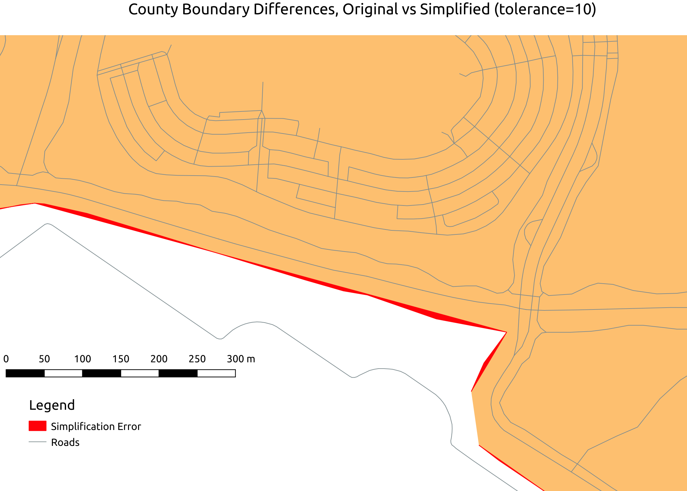
Let's examine a section of The City and County of Broomfield where the errors are the most noticeable in a way that would
affect spatial analysis. The following image was created using
QGIS. It shows a band of red that indicates the area of difference between the original and
the simplified version. That band of red was calculated using the
ST_Difference() function.
This area illustrates pretty much what I saw with all of the differences I observed: long-skinny areas of minor differences.
I say they're minor differences because the "wide" part of the red strip is less than 10 meters across! This is well within the
tolerance and accuracy of many common GIS applications. After reading more about the Douglas-Peucker algorithm
used by ST_Simplify() this pattern makes very good sense.
To see what that area looks like on a zoom-able map, check out the same basic view directly on OpenStreetMap.org.
Assigning points to polygons
A common spatial analysis task is to find points that exist within an area, such as finding businesses within a county. This allows analysts to write queries like: "Show me all the restaurants in Jefferson County." In GIS lingo, this query requires a "spatial join", or a join that takes location into account.
With this type of GIS task in mind, let's use another method to identify errors. We can use the original polygon and the simplified polygon to make the same spatial join and compare the differences. Any differences in the matching between the different layers should be errors.
With OpenStreetMap data already loaded, one convenient source for a lot of points with a random variety of locations is the layer with natural points such as trees, peaks, cliffs, and natural springs. I'm choosing this layer for two reasons, variety and randomness. It has 58,696 rows of data, and the data points represent their natural placements so should be relatively random.
The only way to know how your data will be impacted is to test it out!
The following query counts how many of the natural points match up to both the original county definition and the simplified county definition. This returned 99.7% (58,514) of the natural objects in the database as being residents of their original county!
SELECT COUNT(*)
    FROM osm.natural_point p
    INNER JOIN osm.counties orig ON ST_Intersects(orig.way, p.way)
    INNER JOIN osm.counties_simple1000 simple ON ST_Intersects(simple.way, p.way)
    WHERE orig.osm_id = simple.osm_id
    ;
┌───────┐
│ count │
├───────┤
│ 58514 │
└───────┘
(1 row)
If a 0.3% error rate is a concern, these <200 objects could be manually reviewed without too much overhead.
Performance
One of the main goals with simplifying spatial data is to improve performance. So far I've demonstrated how we can reduce the size on disk
of large polygon objects in PostGIS.
Now, we need to see if this made any difference with a real-world type of query. For this I will run a couple EXPLAIN ANALYZE
queries to compare what PostgreSQL has to do to return my data. The data set returned in both queries is identical and indexes are used
consistently throughout.
These tests were ran on PostgreSQL 9.6 running in a VirtualBox VM with 1 core and 1 GB RAM and a spinning HDD. I ran each query at least twice, taking the second result of each. I know, not the most scientific method for testing performance but should be sufficient to illustrate the task at hand.
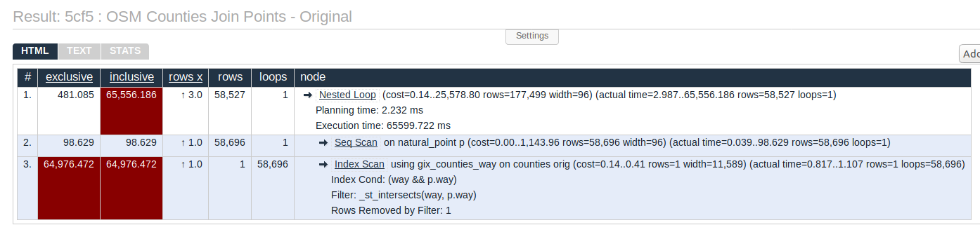
Spatial Join with original counties
The results of the first EXPLAIN ANALYZE (click to see on Explain.Depesz.com) shows that the GIST index is being used. One element to note here
is width=11589 in the join performed in #3. The width is a value in bytes indicating how much data is moving through that step.
Bigger width numbers, in general,
indicates PostgreSQL has to do more work, there's more I/O, and less effective caching due to excessive RAM pressure.
EXPLAIN ANALYZE SELECT p.*
    FROM osm.natural_point p
    INNER JOIN osm.counties orig ON ST_Intersects(orig.way, p.way)
    ;
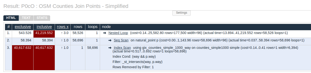
Spatial Join with simplified counties
The results of the simplified geometry query EXPLAIN ANALYZE (click to see on Explain.Depesz.com)
shows the width of that join is down to 6,394, a 45% reduction. That reduction matches the size on disk reduction we saw earlier!
Another thing these two results show is that the simplified version returned 23 seconds quicker,
a 37% reduction in execution time.
The reduction in execution time is not quite as significant as the 45% reduction in disk space. That's because that one column of focus (the one storing the polygon!) is only one factor in that query's overall performance.
EXPLAIN ANALYZE SELECT p.*
    FROM osm.natural_point p
    INNER JOIN osm.counties_simple1000 simple ON ST_Intersects(simple.way, p.way)
    ;
Summary
This post has provided a quick look at the process I've used to simplify spatial data using PostGIS and PostgreSQL.
We examined the affects of simplification of large polygons and how the process might impact spatial analysis.
My findings in this post showed a very small error rate (0.3%) when joining against a point layer.
Considering the errors I found were typically a difference of less than 10 meters, I don't see reason to be overly concerned unless a precision GIS application is in play. Most non-commercial GPS units aren't any more accurate than the errors here, so the accuracy of data at that level must be questioned anyway.
Overall, I believe the benefits to performance and reduction in disk usage far outweigh the minor error rate that is introduced.
The pros:
- 45% reduction in disk space used for large polygons
- 37% reduction in spatial join query times
The cons:
- Found 0.3% error rate from simplification
Need help with your PostgreSQL servers or databases? Contact us to start the conversation!
 Mastodon