
Getting started with MobilityDB
The MobilityDB is an exciting project I have been watching for a while. The project's README explains that MobilityDB "adds support for temporal and spatio-temporal objects." The spatio-temporal part translates as PostGIS plus time which is very interesting stuff to me. I had briefly experimented with the project in its early days and found a lot of potential. Mobility DB 1.0 was released in April 2022, at the time of writing the 1.1.0 alpha release is available.
This post explains how I got started with MobilityDB using PostGIS and pgRouting. I'm using OpenStreetMap roads data with pgRouting to generate trajectories. If you have gpx traces or other time-aware PostGIS data handy, those could be used in place of the routes I create with pgRouting.
Install MobilityDB
When I started working on this post a few weeks ago I had an unexpectedly
difficult time trying to get MobilityDB working.
I was trying to install from the production branch with Postgres 15 and Ubuntu 22.04
and ran into a series of errors. It turned out the fixes
to allow MobilityDB to work with these latest versions had been in the develop
branch for more than a year.
After realizing what the problem was I asked a question and got an answer. The fixes are now in the master branch
tagged as 1.1.0 alpha.
Thank you to everyone involved with making that happen!
To install MobilityDB I'm following the instructions to install from source. These steps involve git clone
then using cmake, make, and sudo make install.
Esteban Zimanyi explained
they are working on getting packaging worked out for providing deb and yum installers.
It looks like work is progressing on those!
Update Configuration
After installing the extension, the postgresql.conf needs to be updated to include
PostGIS in the shared_preload_libraries and increase the max_locks_per_transaction
to double the default value.
shared_preload_libraries = 'postgis-3'
max_locks_per_transaction = 128
I haven't found any explanation in the MobilityDB documentation why
max_locks_per_transactionshould be increased. Per the Postgres documentation: "you might need to raise this value if you have queries that touch many different tables in a single transaction." I also don't see any obvious harm / risk to the change and am following that recommendation for now.
Create extensions
This post uses three (3) extensions, PostGIS, pgRouting and Mobility DB. The following queries create these prerequisites in the target database.
CREATE EXTENSION postgis;
CREATE EXTENSION pgrouting;
CREATE EXTENSION mobilitydb;
Data used
This post uses the same approach as my prior
Trajectories in PostGIS post. A number of
improvements have happened between 2020 when that post was written and now.
Loading OpenStreetMap data is now done with PgOSM Flex
instead of our now-outdated PgOSM project.
The PgOSM Flex project results in far more usable routing data in osm.road_line
compared to the legacy project.
The PgOSM Flex version of osm.road_line has route_motor, route_cycle,
and route_foot columns to which improve common routing logic.
To see how PgOSM Flex implements access control, explore the routable_motor() function. Note the logic uses tags from the
access,motor_vehicle, andhighwaykeys from OpenStreetMap. Theroutable_cycle()androutable_foot()functions are defined in the same Lua script used to calculate theroute_cycleandroute_footcolumns inosm.road_line.
The following query from osm.pgosm_flex shows the region, dates and PgOSM Flex version
used. Version check functions are included for the three (3) extensions being used.
Be aware that the MobilityDB version is reporting v1.1.0, though I am currently
using the Alpha version.
SELECT osm_date, region, srid, pgosm_flex_version,
        postgis_version(), pgr_version(), mobilitydb_version()
    FROM osm.pgosm_flex
    ORDER BY imported DESC
    LIMIT 1
;

┌─[ RECORD 1 ]───────┬───────────────────────────────────────┐
│ osm_date           │ 2023-07-31                            │
│ region             │ north-america/us-colorado             │
│ srid               │ 3857                                  │
│ pgosm_flex_version │ 0.10.0-e7d967e                        │
│ postgis_version    │ 3.3 USE_GEOS=1 USE_PROJ=1 USE_STATS=1 │
│ pgr_version        │ 3.5.0                                 │
│ mobilitydb_version │ MobilityDB 1.1.0                      │
└────────────────────┴───────────────────────────────────────┘
Note: This section is quite lengthy to illustrate how I prepared data for use with MobilityDB. If you want to see how MobilityDB can be used, skip to the Mobility in Action section below.
Routing Costs
Creating routes with pgRouting requires a cost to determine the lowest cost route.
Since time is a big aspect of MobilityDB, I am using time to travel, in minutes, as my main cost.
Forward and reverse costs are calculated using CASE statements like the following
snippet. The CASE statement for the reverse cost (not shown) uses cost_length_reverse
instead of cost_length. The cost_length column is a
simple ST_Length() calculation.
-- Motorized cost in travel time - forward
CASE WHEN r.route_motor
    THEN rn.cost_length / (COALESCE(r.maxspeed, pr.maxspeed) / 60 * 1000)
    ELSE -1
    END AS cost_minutes_motor,
This post cannot get into the depths of preparing the data for routing. My most complete resource on pgRouting spans 4 chapters of my book Mastering PostGIS and OpenStreetMap. See our other blog posts on pgRouting for additional resources on the topic.
Routes
After the data is prepared for pgRouting, the vertices (points) to use for start
and end points in routing are in the routing.road_line_noded_vertices_pgr table.
The following query saves 30 random vertices for start/end points to the
points temp table.
CREATE TEMP TABLE points AS
SELECT id
    FROM routing.road_line_noded_vertices_pgr
    ORDER BY random()
    LIMIT 30
;
The points data is split into two groups by making the rows with even id values
into start_id values, and and rows with odd id values become the end_id values.
The following query saves this data into the start_end_points temp table.
The exact number of rows returned by the query will vary based on the random
start and end points selected. Running this query three times returned
200, 216, and 221 rows.
The second part of the CTE query below
creates a new id column and assigns the start time for each route. The basis
for the ts column is NOW(), with a random number of minutes between 0 and 10
minutes being added to the start time.
CREATE TEMP TABLE start_end_points AS
WITH split AS (
SELECT id, id % 2 AS grp
    FROM points
)
SELECT ROW_NUMBER() OVER () AS id,
        l.id AS start_id, r.id AS end_id,
        NOW() + (((random() * 10)::NUMERIC(4,2))::TEXT || ' minutes')::INTERVAL
            AS ts
    FROM split l
    JOIN split r ON l.grp = 0 AND r.grp = 1
;
The next query creates the routes using
the pgr_dijkstra()
function from pgRouting.
The routes are saved with each step for each route as its own row into
the routing.route_steps table.
It is highly unlikely that all of the 200 input rows from start_end_points will have
routes suitable for motorized traffic.
From the 200 inputs I used, I ended up with 70 routes.
Warning: This query gets increasingly slow as the input row count increases. It took my laptop about 2 minutes to create this table.
CREATE TABLE routing.route_steps AS
SELECT s.id AS route_id,
        -- For each step, add the agg_cost in minutes to the route's start time
        s.ts + (d.agg_cost::TEXT || ' minutes')::INTERVAL AS ts,
        d.*, n.the_geom AS node_geom, e.geom AS edge_geom
    FROM start_end_points s
    -- This function creates the routes by defining the query for routes, plus start/end points
    JOIN pgr_dijkstra(
        'SELECT n.id, n.source, n.target, n.cost_minutes_motor AS cost,
                n.cost_minutes_motor_reverse AS reverse_cost,
                n.geom
            FROM routing.road_line_noded n
            INNER JOIN routing.road_line r ON n.old_id = r.id
                    AND r.route_motor
            ',
            s.start_id, s.end_id, directed := True
        ) d ON True
    -- Joins used to get details about nodes & edges
    INNER JOIN routing.road_line_noded_vertices_pgr n ON d.node = n.id
    LEFT JOIN routing.road_line_noded e ON d.edge = e.id
    ORDER BY s.id, d.seq
;
The following query shows how many routes were created and how many total steps
are involved. The 70 routes I generated resulted in 17,527 node/edge pairs.
The nodes are used along with the ts values to build the trajectories.
The edges are used for PostGIS visualization in this example, in real-world examples
it's common to use the edges to label directions (continue on 1st Street...)
or provide additional details.
SELECT COUNT(DISTINCT route_id) AS route_count,
        COUNT(*) AS route_step_count,
        COUNT(*) / COUNT(DISTINCT route_id) AS avg_steps_per_route
    FROM routing.route_steps
;

┌─────────────┬──────────────────┬─────────────────────┐
│ route_count │ route_step_count │ avg_steps_per_route │
╞═════════════╪══════════════════╪═════════════════════╡
│          70 │            17527 │                 250 │
└─────────────┴──────────────────┴─────────────────────┘
Data so far...
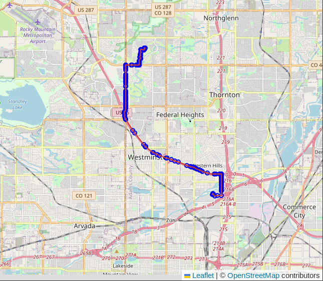
The route with route_id = 1 is shown in the screenshot below. This particular
route has 180 steps (rows) with each step having a node and edge.
SELECT *
    FROM routing.route_steps
    WHERE route_id = 1
;
The first step in route_id = 1 is shown in the table below. The values in
start_vid, end_vid, and node each match rows with points in the
routing.road_line_noded_vertices_pgr table. The edge value relates
to the id in the routing.road_line_noded table. The cost column has the
cost in minutes for the current step, and the agg_cost has the total cost
of all steps up to, but not including, the current step. Since this is the
first step of the route, the agg_cost is 0.
┌─[ RECORD 1 ]───┬─────────────────────────────────────────────────────────────────────────────────┐
│ route_id       │ 1                                                                               │
│ ts             │ 2023-08-09 19:37:31.330503-06                                                   │
│ seq            │ 1                                                                               │
│ path_seq       │ 1                                                                               │
│ start_vid      │ 225854                                                                          │
│ end_vid        │ 295807                                                                          │
│ node           │ 225854                                                                          │
│ edge           │ 290544                                                                          │
│ cost           │ 0.15375990043338703                                                             │
│ agg_cost       │ 0                                                                               │
└────────────────┴─────────────────────────────────────────────────────────────────────────────────┘
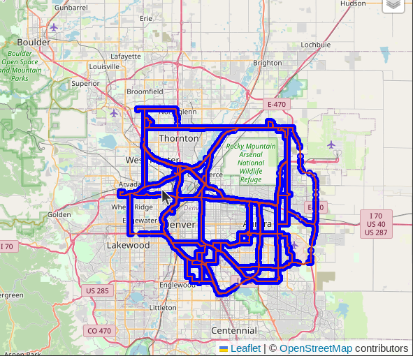
The next screenshot shows a more complete view of the created routes. There is a lot of overlap in these routes due to the method of selecting and pairing the start/end nodes. This is the data we'll be working with in the next sections.
TGEOMPOINT = Point plus Time
The data created in routing.route_steps has a point and a timestamp for each
row. These two columns can be combined with MobilityDB into a TGEOMPOINT.
The following query creates a generated column
that combines the node_geom and ts columns into a TGEOMPOINT
using tgeompoint_inst(). The MobilityDB functions to create these objects are
explained here.
The base of the function name (tgeompoint) aligns with the target data type.
The _inst suffix means it's an "instant". Other options are _instset,
_seq, and _seqset.
ALTER TABLE routing.route_steps
    ADD node_geom_inst TGEOMPOINT NOT NULL
    GENERATED ALWAYS AS (tgeompoint_inst(node_geom, ts)
        ) STORED
;
Now that the routing.route_steps has a node_geom_inst column, the
next step is to aggregate the individual route steps into one row per route.
The following query uses a method I commonly used with standard PostGIS data.
Using ST_Collect()
aggregates the node and edge geometries into respective MULTI geometry type.
To aggregate the new TGEOMPOINT data, the node_geom_inst column is first aggregated
using Postgres' built-in array_agg(), ordering the points by the ts column.
The array of tgeompoint data is then passed into tgeompoint_seq() to create the
sequence of data. The column is named trip here, though in future work I doubt that
is what I'll continue naming it.
CREATE TABLE routing.route_aggregates AS
SELECT route_id,
        -- Non-spatial aggregates
        COUNT(*) AS sequence_count,
        MIN(ts) AS route_start,
        MAX(ts) AS route_end,
        SUM(cost) AS total_cost_minutes,
        -- Aggregate nodes and edges using standard geometry collections
        ST_Collect(node_geom) AS node_geom,
        ST_Collect(edge_geom) AS edge_geom,
        -- MobilityDB
        tgeompoint_seq(array_agg(node_geom_inst
                        ORDER BY ts)
                    ) AS trip
    FROM routing.route_steps
    GROUP BY route_id
    ORDER BY route_id
;
Users familiar with PostGIS will feel at home creating
a GIST index on the trip column.
CREATE INDEX gix_route_steps_trip
    ON routing.route_aggregates USING GIST (trip);
MobilityDB in Action
To summarize the above data preparation steps... I ended up with 70 routes suitable
for motorized traffic stored in the routing.route_aggregates table.
The data includes traditional PostGIS
elements as well as the new MobilityDB-enabled trip column, storing a sequence of
tgeompoint values. The 70 routes have a total of 17,527 steps which are
available with node and edge geometries in routing.route_steps.
Smallest distance
The first MobilityDB operator we'll explore is |=| for smallest distance.
The |=| operator returns the numeric value of the
smallest distance
between two trajectories. The |=| operator takes both time and space into
consideration to determine this smallest distance value.
The following query sets route_id = 1 as a focus. The join searches
for other routes that end up passing within 1000 meters of the focus route.
The query returns six (6) routes sorted by smallest_distance.
SELECT focus.route_id AS focus_route_id, nearby.route_id,
        focus.trip |=| nearby.trip AS smallest_distance
    FROM routing.route_aggregates focus
    INNER JOIN routing.route_aggregates nearby
        ON focus.route_id <> nearby.route_id
            AND focus.trip |=| nearby.trip < 1000
    WHERE focus.route_id = 1
    ORDER BY focus.trip |=| nearby.trip
;
The first five (5) routes are between 27 and 61 meters apart. These are routes passing each other in opposite directions, such as one car traveling north and another traveling south on the same highway. The 6th route are two routes in nearby, but different areas.
┌────────────────┬──────────┬────────────────────┐
│ focus_route_id │ route_id │ smallest_distance  │
╞════════════════╪══════════╪════════════════════╡
│              1 │      198 │ 26.716733679934347 │
│              1 │      193 │  28.77658889081568 │
│              1 │      195 │  35.62986009228122 │
│              1 │      192 │  35.77918844510394 │
│              1 │      200 │  61.22491663877252 │
│              1 │        5 │  657.8665915750265 │
└────────────────┴──────────┴────────────────────┘
These routes are visualized and animated using QGIS' temporal support in the following GIF. Route ID 1 is represented by the red dots that start just southwest of center of the image then travel northwest along CO-36. Most of the nearby routes pass Route ID 1 on the highway, while one route happens to start its route near the beginning of Route ID 1.
It is worth noting that the visualization
was created from the standard PostGIS data stored in routing.route_steps,
not the MobilityDB formatted data.
Points at Smallest Distance
The previous query showed how to use the |=| operator to return the smallest
distance between two MobilityDB trajectories. The next query builds on this
by adding two calls to
nearestApproachInstant().
The nearestApproachInstant() function calculates the closest_focus_geom
and closest_nearby_geom columns. Both columns are cast to geometry via ::GEOMETRY.
This step allows rendering the points in DBeaver, shown in the next screenshots.
SELECT focus.route_id AS focus_route_id, nearby.route_id,
        focus.trip |=| nearby.trip AS smallest_distance,
        -- Order matters of columns, first shows closest point on A
        nearestApproachInstant(focus.trip, nearby.trip)::GEOMETRY AS closest_focus_geom,
        -- Second shows closest point on B
        nearestApproachInstant(nearby.trip, focus.trip)::GEOMETRY AS closest_nearby_geom
    FROM routing.route_aggregates focus
    INNER JOIN routing.route_aggregates nearby
        ON focus.route_id <> nearby.route_id
            AND focus.trip |=| nearby.trip < 1000
    WHERE focus.route_id = 1
    ORDER BY focus.trip |=| nearby.trip
;
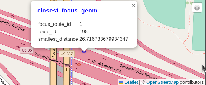
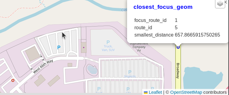
The following screenshot shows the closest points between routes 1 and 198, with 27 meters between them. The screenshot shows the closest focus point as a blue dot and the closest nearby point as a red dot, traveling in opposite directions on U.S. Highway 36.
The next screenshot shows the nearest points between routes 1 and 5. This matched pair is still within the 1000 meter limit, but considerably further away than the other 5 points which were generally found passing each other on the highway. In this example, the focus route was traveling on Broadway, while the nearby point was on a service road in the industrial area to the southwest, 658 meters away. These are the nearby starting points visualized in the above GIF in the Smallest Distance section.
Plenty More to Explore
This post illustrates the very basics of what is available with MobilityDB.
Trajectory data created by pgRouting is clearly an option for the basis of a wide variety of
data modeling projects, such as traffic scenarios.
MobilityDB can also be used with gpx trace data tracking actual trips, with GPS
traces from drone flights, or any number of other GPS-enabled sensors.
The documentation on functions and operators
gives an idea of the features available, such as the speed()
and time-weighted centroid (twcentroid()) functions.
Shameless plug: I'm providing a full day pre-con session at PASS 2023 in November! A lot of topics from this post will be discussed in more depth during this session. I'll also be giving a general session talk about the power of extensions in Postgres. I hope to see you there!
Need help with your PostgreSQL servers or databases? Contact us to start the conversation!
 Mastodon