Better OpenStreetMap places in PostGIS

Data quality is important. This post continues exploring the improved quality of OpenStreetMap data loaded to Postgres/PostGIS via PgOSM-Flex. These improvements are enabled by the new flex output of osm2pgsql, making it easier to understand and consume OpenStreetMap data for analytic purposes.

I started exploring the Flex output a few weeks ago, the post before this one used PgOSM-Flex v0.0.3. This post uses PgOSM-Flex v0.0.7 and highlights a few cool improvements by exploring the OSM place data. Some of the improvements made of the past few weeks were ideas brought over from the legacy PgOSM project. Other improvements were spurred by questions and conversations with the community, such as the nested admin polygons.

Improved places

This post focuses on the osm.place_polygon data that stores things like city, county and Country boundaries, along with neighborhoods and other details. The the format of place data has a number of improvements covered in this post:

• Consolidated name
• Remove duplication between relation/member polygons
• Boundary hierarchy

The data loaded for this post is the U.S. West sub-region from Geofabrik. It was loaded using the run-all.lua and run-all.sql scripts in PgOSM-Flex.

This post is part of the series PostgreSQL: From Idea to Database.

Consolidated Name

There are a variety of name tags used throughout various OSM features, such as name, alt_name, short_name, and so on. Since not all features are tagged equally, the name cleanup implemented in helpers.lua attemps to catch the majority of the name tags used. The get_name(tags) function is used for the name column in every layer throughout PgOSM-Flex, not just the place layers.

function get_name(tags)
    if tags.name then
        return tags.name
    elseif tags.short_name then
        return tags.short_name
    elseif tags.alt_name then
        return tags.alt_name
    elseif tags.loc_name then
        ...

This query shows more than 4,500 roads that end up with a value in name that otherwise be missing.

SELECT COUNT(*)
    FROM osm.road_line r
    INNER JOIN osm.tags t
        ON t.geom_type = 'W' AND r.osm_id = t.osm_id
            AND t.tags->>'name' IS NULL -- The main name tag is empty
    WHERE r.name IS NOT NULL -- The road has a name
;

┌───────┐
│ count │
╞═══════╡
│  4585 │
└───────┘

The above query takes advantage of the osm.tags table that stores every feature with its full set of unaltered tag data. osm.tags is the largest object loaded by PgOSM-Flex, considerable size can be saved by using run-no-tags.lua instead of run-all.lua.

Also, of note, is the use of JSONB instead of HSTORE throughout PgOSM-Flex. The osm2pgsql project is still defaulting to HSTORE for legacy reasons.

Relations and Member Polygons

Many administrative boundaries have multiple parts making up their complex shapes. This results in the full relation polygon and multiple sub-parts being loaded into PostGIS. This query looking for Golden, CO returns two rows instead of the expected one.

SELECT osm_id, osm_type, boundary, admin_level, name, member_ids
    FROM osm.place_polygon p
    WHERE p.name = 'Golden'
    ORDER BY osm_id;

Note the the osm_id in the second row is listed in the member_ids column of the first row. The negative ID value (osm_id = -112204) indicates that row is a relation while the other is a way.

┌──────────┬──────────┬────────────────┬─────────────┬────────┬──────────────────────┐
│  osm_id  │ osm_type │    boundary    │ admin_level │  name  │      member_ids      │
╞══════════╪══════════╪════════════════╪═════════════╪════════╪══════════════════════╡
│  -112204 │ city     │ administrative │           8 │ Golden │ [33113240, 33113235] │
│ 33113240 │ city     │ administrative │           8 │ Golden │ ¤                    │
└──────────┴──────────┴────────────────┴─────────────┴────────┴──────────────────────┘

The legacy osm2pgsql process did not make it easy to remove the component geometries, at least not that I found. When using this data for analysis, this resulted in duplication that generally required manual cleanup.

The member_ids column shown above is pulled in during osm2pgsql processing by the place.lua style. The tables get a new column defined:

{ column = 'member_ids', type = 'jsonb'},

The processing uses the way_member_ids() function.

local member_ids = osm2pgsql.way_member_ids(object)

WARNING: The view osm.vplace_polygon was removed in PgOSM Flex 0.6.0. In modern PgOSM Flex versions the cleanup done by this view is done directly in the osm.place_polygon table. This post is accurate for the version of PgOSM Flex it was written against.

The associated post-processing SQL script (place.sql) creates a view osm.places_in_relations that is then used to create the materialized view osm.vplace_polygon.

Querying osm.vplace_polygon only returns the one relation result for Golden, CO.

SELECT osm_id, osm_type, boundary, admin_level, name, member_ids
    FROM osm.vplace_polygon p
    WHERE p.name = 'Golden'
    ORDER BY osm_id;

┌─────────┬──────────┬────────────────┬─────────────┬────────┬──────────────────────┐
│ osm_id  │ osm_type │    boundary    │ admin_level │  name  │      member_ids      │
╞═════════╪══════════╪════════════════╪═════════════╪════════╪══════════════════════╡
│ -112204 │ city     │ administrative │           8 │ Golden │ [33113240, 33113235] │
└─────────┴──────────┴────────────────┴─────────────┴────────┴──────────────────────┘

How big of a deal this is will vary greatly on your region's data and how you are querying it. In the case of U.S. West, removing rows included in relations cuts out 23% of the table's total row count.

WITH aggs AS (
SELECT COUNT(*) FILTER (
            WHERE NOT EXISTS (
                SELECT 1
                    FROM osm.vplace_polygon p
                    WHERE p_full.osm_id = p.osm_id)
        ) AS polys_removed,
        COUNT(*) AS total_polys
    FROM osm.place_polygon p_full
)
SELECT *, ROUND(polys_removed * 100. / total_polys, 0)::TEXT || '%' AS percent_removed
    FROM aggs
    ;

┌───────────────┬─────────────┬─────────────────┐
│ polys_removed │ total_polys │ percent_removed │
╞═══════════════╪═════════════╪═════════════════╡
│          5982 │       26154 │ 23%             │
└───────────────┴─────────────┴─────────────────┘

Nested places

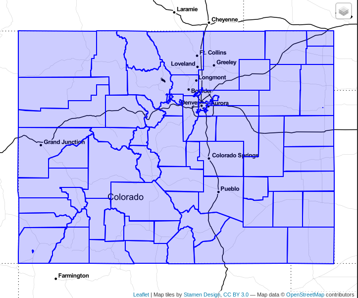
Nested places refers to administrative boundaries that are contained, or contain, other administrative boundaries. An example of this is the State of Colorado contains the boundary for Jefferson County, Colorado. Determining these hierarchical structures can be accomplished in PostGIS using spatial joins, using ST_Contains() or ST_Within(). An example of a query using ST_Within() is below.

EXPLAIN (ANALYZE, BUFFERS, VERBOSE)
SELECT cn.*
    FROM osm.vplace_polygon st -- State  
    INNER JOIN osm.vplace_polygon cn -- County
        ON ST_Within(cn.geom, st.geom) AND cn.admin_level::INT = 6
    WHERE st.name = 'Colorado'
;

My laptop runs this query in 57 ms (22 ms planning + 54 ms execution). The EXPLAIN output shows the spatial index scan is the most time consuming step, taking more than 40 ms.

Index Scan using gix_osm_vplace_polygon ... (actual time=3.497..43.628 rows=69 loops=1)

A screenshot to visualize the results from the above query because pictures are nice.

Note: An astute reader may notice the name column is not indexed, indicated by the Seq Scan portion of the plan. The Seq Scan took 9 ms, replacing it with an index scan reduced that step (and the overall query) by only 4-5 ms. As the next section shows, this still falls short on performance.

Prepare the nested data

The nested data is in the table osm.place_polygon_nested but does not have the nesting details calculated during the main processing steps. The columns nest_level, name_path, osm_id_path and admin_level_path are all NULL to start, and the row_innermost and innermost columns are all False.

The procedure (osm.build_nested_admin_polygons()) is created but not executed by default with the PgOSM-Flex scripts. This process runs really fast on small regions (e.g. Colorado) but can take quite a while (> 1 hour) on larger regions (Europe). Due to the non-negligible processing time on large regions, and the fact that not everyone will use this data, I decided to skip this in the default processing for now.

Log into the pgosm database and run the procedure:

CALL osm.build_nested_admin_polygons();

This calculates the nesting of each row in small batches, default batch size 100. After each batch runs it is committed. Once all rows have processed, the final steps calculate a boolean innermost column to easily identify boundaries that do not contain other boundaries, e.g. the narrowest, most focused boundaries.

Running this UPDATE process in batches allows incremental processing to spread out load over a longer time on large regions being loaded on busy servers. It also allows monitoring the long running process.

A look at the nested data with this query.

SELECT osm_id, name, osm_type, name_path
    FROM osm.place_polygon_nested n
    WHERE innermost 
        AND ARRAY['Colorado'] && name_path
    ORDER BY nest_level DESC, name_path Desc
    LIMIT 5
;

This query uses && to filter on name_path checking for overlap with another array. Using ARRAY['Colorado'] makes it easy to update to include multiples, such as ARRAY['Colorado', 'Utah'].

┌───────────┬────────────────────────────────────┬──────────┬────────────────────────────────────────┐
│  osm_id   │                name                │ osm_type │               name_path                │
╞═══════════╪════════════════════════════════════╪══════════╪════════════════════════════════════════╡
│   -113214 │ Orchard Mesa                       │ locality │ {Colorado,"Mesa County","Orchard Mesa"…│
│           │                                    │          │…,"Orchard Mesa"}                       │
│  33123135 │ Sunburst Knoll (Historical)        │ boundary │ {Colorado,"Larimer County","Fort Colli…│
│           │                                    │          │…ns","Sunburst Knoll (Historical)"}     │
│  33123153 │ Southwest Enclave Phase 3, part 3 …│ boundary │ {Colorado,"Larimer County","Fort Colli…│
│           │…of 3 (historical)                  │          │…ns","Southwest Enclave Phase 3, part 3…│
│           │                                    │          │… of 3 (historical)"}                   │
│  33123152 │ Fossil Creek Annexation (historica…│ boundary │ {Colorado,"Larimer County","Fort Colli…│
│           │…l)                                 │          │…ns","Fossil Creek Annexation (historic…│
│           │                                    │          │…al)"}                                  │
│ 761924569 │ Coyote Ridge II, SW Enclave III & …│ boundary │ {Colorado,"Larimer County","Fort Colli…│
│           │…IV, Cathy Fromme II (historical)   │          │…ns","Coyote Ridge II, SW Enclave III &…│
│           │                                    │          │… IV, Cathy Fromme II (historical)"}    │
└───────────┴────────────────────────────────────┴──────────┴────────────────────────────────────────┘

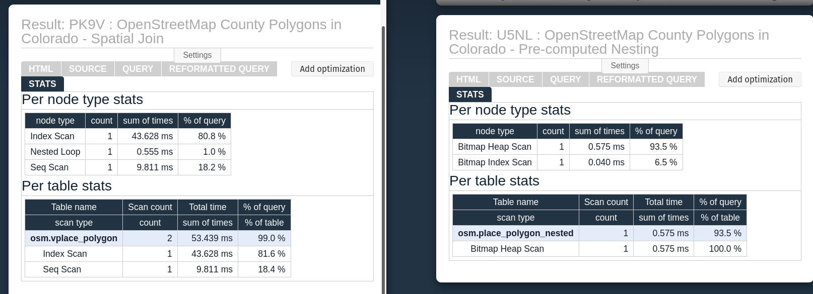
Faster County in State query

Below is the new query for finding counties of Colorado using the pre-calculated nesting. This query no longer requires a spatial self-join, and should remove the most expensive step of the query. Now the containment search uses the GIN index on the name_path column.

The original version of this query took 57 ms. This query takes 1 ms (.4 ms planning + .6 ms execution), or 98% faster! See the full plan.

-- Counties in Colorado - New way
EXPLAIN (ANALYZE, BUFFERS, VERBOSE)
SELECT n.*
    FROM osm.place_polygon_nested n
    WHERE ARRAY['Colorado'] && name_path
        AND admin_level::INT = 6
;

The following screenshot shows the two query plan's Stats tables side by side, the original on the left and the new on the right. This helps illustrate difference in timing and complexity that isn't always as easy to see in the pure textual output.

Bonus: Reproduce and Share

An improvement not directly related to the OpenStreetMap data itself is the PgOSM-Flex project now tracks meta-data related to the processing of the data. The osm.pgosm_flex table has one row with this information. The pgosm_flex_version tracks the latest tag from Git and the current commit hash. The srid is customizable at run-time so that is captured as well. The osm2pgsql_version will inevitably change over time.
The ts is currently the timestamp (using Postgres' timezone setting) indicating when the associated .sql script was ran. I plan to get that column handled in the Lua script eventually.

SELECT * 
    FROM osm.pgosm_flex;


┌─[ RECORD 1 ]───────┬─────────────────────────────────────────────┐
│ pgosm_flex_version │ 0.0.7-3d3d9a4                               │
│ srid               │ 3857                                        │
│ project_url        │ https://github.com/rustprooflabs/pgosm-flex │
│ osm2pgsql_version  │ 1.4.0                                       │
│ ts                 │ 2021-01-23 15:09:56.813747+00               │
└────────────────────┴─────────────────────────────────────────────┘

The SRID can also be extracted from the data itself using the ST_SRID() function, such as SELECT DISTINCT ST_SRID(geom) FROM osm.place_polygon;. It was easy to add to the table above and the cost of storing it is essentially nothing.

Summary

This post has covered a few distinct improvements to the quality of the OpenStreetMap place data within PostGIS. While the osm2pgsql flex output is still considered experimental, I can only recommend moving forward with using the Flex output and ditching the old method. I'm sure the PgOSM-Flex project in its current form is only scratching the surface of what can be done. My focus so far has been re-implementing my most-used structures from the legacy PgOSM project. The goal for PgOSM-Flex now is switching to continue with new improvements! If you have ideas or notice bugs please report an issue!

Need help with your PostgreSQL servers or databases? Contact us to start the conversation!