
Scaling osm2pgsql: Process and costs
I love working with OpenStreetMap (OSM) data in PostGIS. In fact, that combo
is the main reason I made the leap to Postgres a few years ago!
One downside? Getting data through osm2pgsql takes a bit of patience
and can require quite a bit of Oomph from the system doing the load.
Earlier this year I wrote about this process for smaller regions using a
local virtual machine
and the Raspberry Pi 3B.
While small area extracts, such as Colorado, are great for some projects,
other projects require much larger data sets. Larger data sets
can benefit from (or even require!) more powerful hardware.
As OSM's PBF file approaches and exceeds 1GB the process starts requiring some serious RAM in order to complete the process. Testing this process in depth got me curious about cost effectiveness and time involved to load OpenStreetMap data as the source data size increases. I know that I can spool up a larger instance and the process will run faster, but does it end up being cheaper? Or just faster? This post is an attempt to document what I have found.
This post is part of the series PostgreSQL: From Idea to Database. Also, see our recorded session Load PostGIS with osm2pgsql for similar content in video format.
Systems tested
Four systems from Digital Ocean were tested for this post, each running Ubuntu 18.04 with PostgreSQL 11 and PostGIS 2.5.
I chose Digital Ocean droplets for two main reasons:
- Transparent pricing
- Fast SSDs
Transparent pricing is important since a main goal is calculating
cost of processing, the second is important because I/O speed
is hugely important for osm2pgsql
processing. The table below has the important details for each machine tested,
affectionately named "Rig A" through "Rig D".
Note: Rigs A through C are "General Purpose" droplets with shared CPU. Rig D is a memory optimized Droplet with dedicated CPUs.
| Name | $ Cost (month / hourly) | # CPUs | RAM (GB) | SSD Disk (GB) |
|---|---|---|---|---|
| Rig A | $20/mo ($0.03/hr) | 2 | 4 | 80 |
| Rig B | $40/mo ($0.06/hr) | 4 | 8 (+20GB SWAP) | 160 |
| Rig C | $160/mo ($0.238/hr) | 8 | 32 (+20GB SWAP) | 640 |
| Rig D | $880/mo ($1.31/hr) | 16 | 128 | 1,200 |
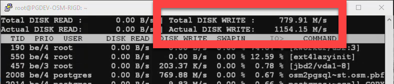
Fast SSDs
I consider Digital Ocean's SSDs fast enough based on repeated observations from
iotop like the following screenshot. Rig D was the only one I observed
able to push data to disk this quickly, the others seemed to peak
between 400-500 M/s. (I know, that's all, right?!)
Why so much SWAP?
A significant amount (20GB) of
SWAP
is indicated on two configurations, Rig B and Rig C. The additional SWAP
provides enough total available RAM to prevent osm2pgsql from crashing
during the larger load processes.
Rig B didn't have enough RAM to load U.S. West or North America without the additional swap. I've found U.S. West requires roughly 15 GB available and North America and Europe both require roughly 20GB of RAM, hence the SWAP on Rig C as well.
Files to Load
The size of the data being loaded is a major factor to consider for this process. The source files in PBF format reach well into the GB range and when loaded to PostGIS roughly 6x the disk space is required. A major selling point of OSM's PBF format (available from Geofabrik's download server) is its impressive compression ratio. The following table illustrates the sizes of the source PBF file and the rough expected size in PostGIS.
| Region | PBF Size | PostGIS Size |
|---|---|---|
| Washington D.C. | 15.9 MB | 129 MB |
| Colorado | 181 MB | 1 GB |
| California | 817 MB | 4.7 GB |
| U.S. West | 1.7 GB | 9.7 GB |
| North America | 8.7 GB | 46 GB |
| Europe | 20.4 GB | 138 GB |
Not all files were tested on the two smaller systems. This is mostly due to limitations to built-in disk capacity of the droplets. While it is possible to add block storage devices for additional capacity, that makes configuration and cost calculations more complex.
The process
My approach to using osm2pgsql is to run the process on a temporary server
used for this one and only task.
Setup
It's critical to automate the deployment of servers. Our deployments are
automated with Ansible
to install and configure the
server. The process takes roughly 10 minutes regardless of how powerful
the server is. apt upgrade and apt install postgresql-11 (etc) don't
get much faster, regardless of how much power you have available...
The other main setup step is to download the PBF file from Geofabrik to process. This time is dependent on network speed and file size, for the sake of this analysis we estimate a flat 5 minutes for this step.
Ansible deployment + wget PBF brings the setup time to 15 minutes.
Processing
Run osm2pgsql. The following command is a good starting point
for smaller imports under 1GB PBF.
osm2pgsql --create --slim --drop \
  --hstore --multi-geometry \
  -d pgosm district-of-columbia-latest.osm.pbf
For "larger" PBF files it can be helpful to use --flat-nodes.
This uses a nodes_file, essentially a giant file on disk to use to store the
nodes instead of putting them in Postgres. This file is now up to 52 GB 😮, up
from 46 GB in January 2019 (+13%).
The cut point for what makes a "larger" file depends greatly on how
fast your disks are.
In my first osm2pgsql post I defined that cut point
as 15 GB, but that was based on relatively slow spinning HDDs. My testing for this
post showed that cut point is around 1 GB for the super fast SSDs used in
Digital Ocean's droplets.
Note: The
--unloggedoption was removed in version 1.0 ofosm2pgsql, instead automatically enabling this option when--dropis enabled.
Post processing
Once the OpenStreetMap data is loaded into PostGIS post-processing is likely to be required. Examples of post-processing include data quality checks, restructuring data for analysis, preparing for pgrouting, or any number of other things.
Because of the wide variety of options with a wide variety of processing times associated, this analysis will simply add a flat 10 minutes for post-processing. You can easily adjust this number for your own processes to provide a more accurate estimate.
Time to run osm2pgsql
The following table shows the time to run osm2pgsql for each file on
each server. This represents the time to run osm2pgsql only.
N/A indicates the file was not tested on a particular server due to
insufficient built-in disk space.
| Source File | Rig A | Rig B | Rig C | Rig D |
|---|---|---|---|---|
| District of Columbia | 15 s | 14 s | 15 s | 11s |
| Colorado | 121 s | 106 s | 113 s | 78 s |
| California | 30min 55s | 9min 39s | 10min 1s | 6min 32s |
| U.S. West | N/A | 30min | 19min 21s | 11min 24s |
| North America | N/A | 5h 43min | 1h 39min | 60 min 12 s |
| Europe | N/A | N/A | 10h 20m | 4h 5m |
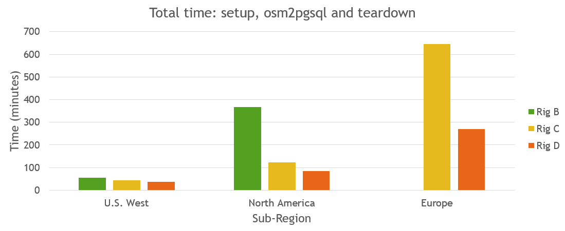
Total time
The following table show the time for osm2pgsql to run for each combination
plus startup time (15 minutes) and teardown (10 minutes). All times rounded to the nearest minute.
| Source File | Rig A | Rig B | Rig C | Rig D |
|---|---|---|---|---|
| District of Columbia | 25 | 25 | 25 | 25 |
| Colorado | 27 | 27 | 27 | 26 |
| California | 56 | 35 | 35 | 31 |
| U.S. West | N/A | 55 | 44 | 36 |
| North America | N/A | 368 | 124 | 85 |
| Europe | N/A | N/A | 645 | 270 |
The following chart visualizes the total processing time for the three larger regions on the three larger test servers, Rigs B - D. Rig B does not have enough built-in storage to process Europe so was not included.
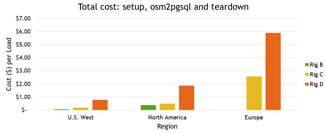
Calculating costs
Using the data outlined above, a total cost was calculated for each file and server.
| Source File | Rig A | Rig B | Rig C | Rig D |
|---|---|---|---|---|
| District of Columbia | $0.01 | $0.03 | $0.10 | $0.55 |
| Colorado | $0.01 | $0.03 | $0.11 | $0.57 |
| California | $0.03 | $0.03 | $0.14 | $0.68 |
| U.S. West | N/A | $0.06 | $0.17 | $0.79 |
| North America | N/A | $0.37 | $0.49 | $1.86 |
| Europe | N/A | N/A | $2.56 | $5.90 |
Summary
As with most things in life, there are trade offs involved. Do you want the end result faster, or the total cost to be cheaper? With patience, even the largest data loads can be coerced to load on small hardware. The trade-off is how long it takes (when it works all) and how long it takes you to get working to a finished product.
In general, throwing more hardware can make it faster but that too has its limits. Looking at D.C. loads, Rig D was the fastest (11 s, $0.55) but Rig A wasn't far behind (15 s) and was a lot cheaper ($0.01). Heck, the Raspberry Pi 3B can complete the D.C. load in only 6 minutes (with a non-app class SD card, none-the-less!).
In the end it comes down to evaluating what your needs are, testing out your options, then optimize from there.
Need help with your PostgreSQL servers or databases?
Contact us to start the conversation!
 Mastodon