Working with GPS data in PostGIS

One of the key elements to using PostGIS is having spatial data to work with! Lucky for us, one big difference today compared to the not-so-distant past is that essentially everyone is carrying a GPS unit with them nearly everywhere. This makes it easy to create your own GPS data that you can then load into PostGIS! This post explores some basics of loading GPS data to PostGIS and cleaning it for use. It turns out, GPS data fr om nearly any GPS-enabled device comes with some... character. Getting from the raw input to usable spatial data takes a bit of effort.

This post starts with using ogr2ogr to load the .gpx data to PostGIS. Once the data is in PostGIS then we actually want to do something with it. Before the data is completely usable, we should spend some time cleaning the data first. Technically you can start querying the data right away, however, I have found there is always data cleanup and processing involved first to make the data truly useful.

This is especially true when using data collected over longer periods of time with a variety of users and data sources.

Travel database project

Before I started writing this post I had assumed that all of the code would be contained in the body of this post. It turned out that to get to the quality I wanted, I had to create a new travel database project (MIT licensed) to share the code. This is already a long post without including a few hundred more lines of code! The travel-db project creates a few tables, a view, and a stored procedure in the travel schema. The stored procedure travel.load_bad_elf_points is responsible for cleaning an importing the data and weighs in at nearly 500 lines of code itself.

Create database and deploy schema

To follow along you need a Postgres database with PostGIS and convert extensions installed. Connect to your instance as a superuser with psql and run the following commands.

CREATE DATABASE travel_demo;
\c travel_demo

CREATE EXTENSION IF NOT EXISTS postgis;

-- See: https://github.com/rustprooflabs/convert
CREATE EXTENSION IF NOT EXISTS convert;

Some queries in this post use the PgDD extension (GitHub). This extension is not required for using the travel database, install if you want.

CREATE EXTENSION IF NOT EXISTS pgdd;

To deploy the travel database schema, clone the project and deploy with Sqitch.

git clone git@github.com:rustprooflabs/travel-db.git
cd travel-db/db
sqitch db:pg:travel_demo deploy

The travel schema is created with a few tables, a view, and a stored procedure to clean and load the data from the ogr2ogr tables. The code in the project currently is targeted to the Bad Elf GPS unit used to the data I've used recently.

Data source

The data sources I'm using for this post are personal GPS traces from a few trips we have taken in 2023. The data was recorded by a Bad Elf GNSS Surveyor unit. What's especially fun about this project for me is it includes data from our travels (already fun!) with four (4) travel methods, by foot, train, car, and airplane. With multiple modes of travel, and knowing each mode of travel has unique nuances, that means I get write a lot of fun queries for different scenarios! 🤓

While I used a Bad Elf unit, there are plenty of apps that can be installed on your phone or table to track your location over time without an additional GPS unit. The apps I have used make it easy to send yourself the trace in .gpx format.

GPX data to PostGIS

This section shows how to load gpx data into PostGIS using the powerful ogr2ogr tool. The first step I take to load GPX data is to drop and recreate the staging schema. This step assumes that the only processes using the staging schema will auto-create their tables, which is easy enough when using ogr2ogr.

psql -d travel -c "DROP SCHEMA IF EXISTS staging CASCADE; CREATE SCHEMA staging;"

The following command uses ogr2ogr to load the Flight-to-PASS-2023.gpx file to the travel database into the staging schema. You can download this GPX file (2.5 MB) for a real-world file to use along with this post.

ogr2ogr -t_srs EPSG:3857 \
    -f "PostgreSQL" PG:"host=localhost dbname=travel" \
    -overwrite -lco SCHEMA=staging \
    /data/badelf/Travel/Seattle-PASS-2023/Flight-to-PASS-2023.gpx

The above command creates a handful of tables, though I am only using one of those tables here. The staging.track_points table has everything I want to work with for this post. The following query using PgDD shows the table has 10,347 rows from the one .gpx file imported.

SELECT s_name, t_name, rows, size_plus_indexes
    FROM dd.tables
    WHERE s_name = 'staging'
        AND t_name = 'track_points'
;

┌─────────┬──────────────┬───────┬───────────────────┐
│ s_name  │    t_name    │ rows  │ size_plus_indexes │
╞═════════╪══════════════╪═══════╪═══════════════════╡
│ staging │ track_points │ 10347 │ 1360 kB           │
└─────────┴──────────────┴───────┴───────────────────┘

At this point, you have some data in the staging schema. Now what? If you visualize the first couple hundred rows in DBeaver you'd notice it appears I was wandering around on the tarmac outside the airport terminal. I promise, I was sitting safely inside in a crowded nook on an uncomfortable and over-worn seat! Instead, the following image skips over those initial points to visualize the points from when the airplane was taxiing and taking off. The following query selects these points based on the ogc_fid column.

SELECT *
    FROM staging.track_points
    WHERE ogc_fid > 1500 AND ogc_fid < 2300
;

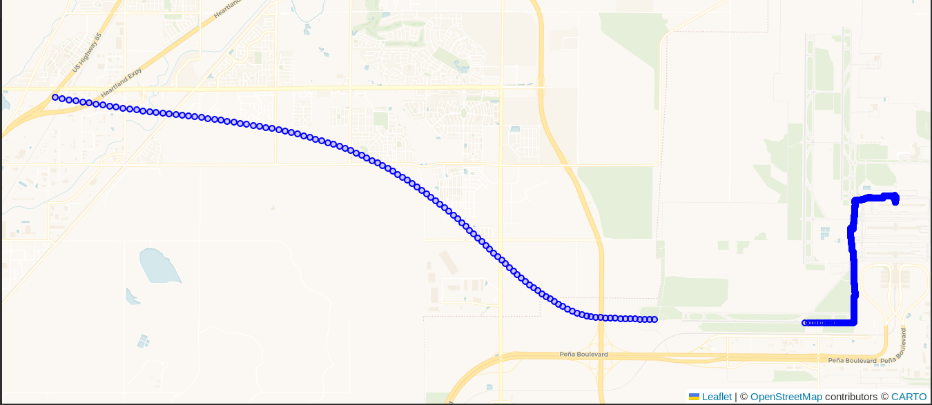
The above screenshot shows the first hint of data quality issues that need to be dealt with: GPS units are far from perfect especially when real humans are using them. There is a 35 second gap between ogc_fid = 2185 and ogc_fid = 2186 during takeoff. This can be seen on the above screenshot in the lower right corner as an obvious gap of missing blue dots. During that time we accelerated from 61.9 m/s to 103.5 m/s (138 mph to 231 mph) and climbed just over 200 meters in elevation. My suspicion is that some combination of the severe acceleration and change in pitch during takeoff caused the Bad Elf to lose track of the satellites.

My Bad Elf was secured in a side pocket of my laptop bag, which was underneath the seat in front of me.

Setting up Travel DB

The previous section showed how to use ogr2ogr to import GPS traces from GPX format into PostGIS. The next sections show how to setup and use our new travel database to import data in way to track more than one trip, with a bit higher data quality and usability.

My goals for this project were to support any number of trips where each trip has one or more legs of travel. Each leg of travel can have one or more steps. To illustrate these components, we'll look closer at our trip to the PASS Summit in November. That trip consisted of everything between leaving home and returning home. The first leg of the trip involved driving from from home to Denver International Airport (DIA), walking through DIA and onto a plane, flying to Seattle's airport (SEATAC), and walking through the airport to get to a taxi to get us to the hotel. I recorded that as four steps to make up one leg of this trip.

In the travel database, the travel.trip detail defines the main trip record. The travel.trip_step table captures the detail of the various legs and steps, where "to Seattle" is a leg, and each mode of travel (car, foot, airplane) is represented as a different step.

Setup records for trips and steps

The following queries setup records in the travel.trip and travel.trip_step tables. The following code uses an anonymous code block to enable setting and re-using the _trip_id variable. The travel.trip_step table defines a timeframe column as a TSTZRANGE. This timeframe column is very important. It is used to match data from the input files (.gpx) to the trip steps. This is helpful in most cases, but may cause points from the input file to be unexpectedly dropped.

DO $$
    DECLARE
        _trip_id BIGINT;
    BEGIN

    WITH add_trip AS (
    INSERT INTO travel.trip (trip_name, timeframe, trip_desc)
        VALUES ('PASS 2023', TSTZRANGE('2023-11-12 00:00:00 -07'::TIMESTAMPTZ,
                                    '2023-12-16 23:59:59 -07'::TIMESTAMPTZ)
                , 'Trip to PASS 2023 to present PostGIS pre-conference session!')
        RETURNING trip_id
    )
    SELECT trip_id INTO _trip_id
        FROM add_trip
    ;

    INSERT INTO travel.trip_step (trip_id, leg_name, step_name, timeframe, travel_mode_id)
    SELECT _trip_id, 'To Seattle', 'At DIA' ,
            '["2023-11-12 10:00:00 -07", "11/12/23 10:39:43 -07")'::TSTZRANGE,
            tm.travel_mode_id
        FROM travel.travel_mode tm
        WHERE tm.travel_mode_name = 'foot'
    UNION
    SELECT _trip_id, 'To Seattle', 'Flight to Seattle',
            '["11/12/23 10:39:43-07", "2023-11-12 13:37:27.000 -07")'::TSTZRANGE,
            tm.travel_mode_id
        FROM travel.travel_mode tm
        WHERE tm.travel_mode_name = 'airplane'

    <add additional UNION queries to setup the remaining steps...>
    ;

END
$$
;

The above code is abbreviated to only show two of the travel.trip_step records. The detail of the other two steps from the shared .gpx file is shown in the following table. If you are following along you'll need to add the other two records to the query above to get the same results.

┌──────────────┬─────────┬────────────┬─────────────────────┬─────────────────────────────────────────────────────┐
│ trip_step_id │ trip_id │  leg_name  │      step_name      │                      timeframe                      │
╞══════════════╪═════════╪════════════╪═════════════════════╪═════════════════════════════════════════════════════╡
│            6 │       1 │ To Seattle │ At DIA              │ ["2023-11-12 10:00:00-07","2023-11-12 10:39:43-07") │
│            8 │       1 │ To Seattle │ Flight to Seattle   │ ["2023-11-12 10:39:43-07","2023-11-12 13:37:27-07") │
│            5 │       1 │ To Seattle │ SEATAC to Taxi      │ ["2023-11-12 13:37:27-07","2023-11-12 13:45:44-07") │
│            7 │       1 │ To Seattle │ Taxi to Grand Hyatt │ ["2023-11-12 13:45:44-07","2023-11-12 14:26:04-07") │
└──────────────┴─────────┴────────────┴─────────────────────┴─────────────────────────────────────────────────────┘

The way I run this step is to create a .sql script containing the commands, then use psql's handy \i command to run the .sql file. The following example illustrates this.

([local] 🐘) ryanlambert@travel_demo=# \i /data/badelf/Travel/Seattle-PASS-2023/trip--setup-pass-2023-records.sql

Run procedure to import

Running the travel.load_bad_elf_points() procedure cleans and imports the raw data from the staging tables into the tables in the travel schema. The following command runs the procedure for trip_id = 1.

CALL travel.load_bad_elf_points(1);

If everything has been setup properly, you should see output similar to the following.

NOTICE:  Ensure data is populated to travel.trip AND travel.trip_step before running this procedure.
NOTICE:  Loading Bad Elf data to points table for Trip ID: 1 (PASS 2023)
NOTICE:  table "trip_cleanup" does not exist, skipping
NOTICE:  table "dup_cleanup_ids" does not exist, skipping
NOTICE:  table "dup_cleanup" does not exist, skipping
NOTICE:  table "dup_remove_ids" does not exist, skipping
NOTICE:  Initial quality check passed...
NOTICE:  table "trip_cleanup_2" does not exist, skipping
NOTICE:  Timestamp gap analysis...
9378 rows
30 greater than 1 second gap
4 greater than 10 seconds gap
1 greater than 60 seconds gap
NOTICE:  Adding data to travel.trip_point
NOTICE:  Building line data and updating travel.trip_step geom.
NOTICE:  Import summary:
9378 points added
Data included covers 4 steps from trip_step. 
4 steps were updated with line geometry
CALL
Time: 2597.017 ms (00:02.597)

Data loaded

The next examples use my local database with four (4) trips loaded and a total of 15 trip steps. The travel.trip_point table now has nearly 100,000 rows, compared to nearly 9,300 from the examples above.

SELECT t_name, rows
    FROM dd.tables
    WHERE s_name = 'travel'
    ORDER BY t_name
;

┌──────────────────────────┬───────┐
│          t_name          │ rows  │
╞══════════════════════════╪═══════╡
│ import_duplicate_cleanup │    51 │
│ travel_mode              │     4 │
│ trip                     │     4 │
│ trip_point               │ 96941 │
│ trip_step                │    15 │
└──────────────────────────┴───────┘

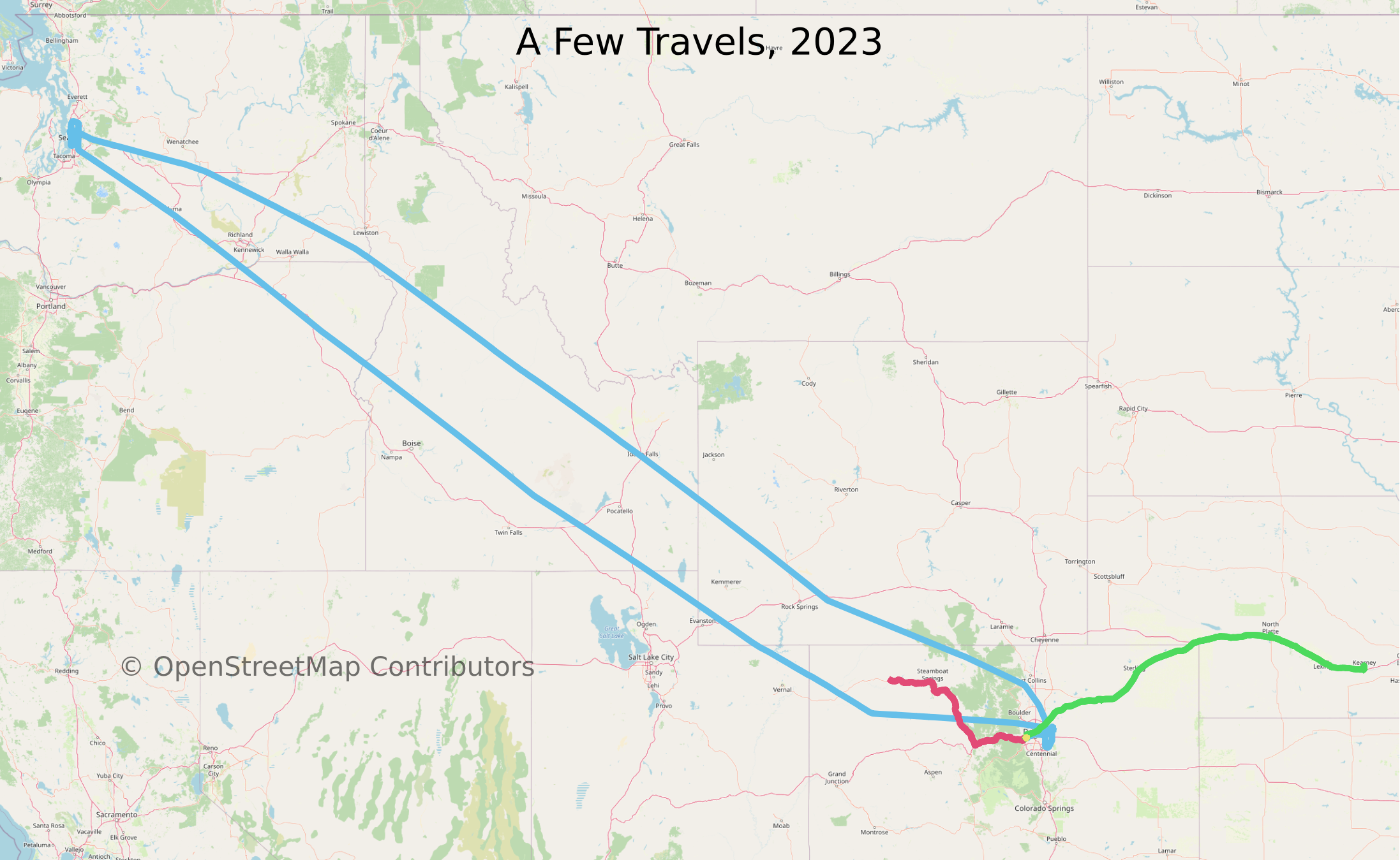
The following image gives an idea of the other travels I am tracking in my database so far.

Aggregated data

The records in travel.trip_step are updated during the import with aggregates from the detailed point data. The following query further aggregates those to grouped by travel_mode_name, sorted by highest max elevation. Air travel naturally was the highest, at nearly 38,000 feet. Motor travel came in second at 11,191 feet, which was from Eisenhower Tunnel. Note, my GPS recorded me driving 33 feet above the highest point.

SELECT tm.travel_mode_name, COUNT(DISTINCT trip_step_id) AS trip_step_count,
        SUM(ST_NPoints(ts.geom)) AS point_count,
        convert.speed_m_s_to_mph(AVG(ts.speed_avg)) AS speed_avg_mph,
        convert.speed_m_s_to_mph(AVG(ts.speed_avg_moving)) AS speed_avg_moving_mph,
        convert.dist_m_to_ft(MIN(ts.ele_min)) AS ele_min_ft,
        convert.dist_m_to_ft(MAX(ts.ele_max)) AS ele_max_ft
    FROM travel.trip_step ts
    INNER JOIN travel.travel_mode tm ON ts.travel_mode_id = tm.travel_mode_id
    GROUP BY tm.travel_mode_name
    ORDER BY ele_max_ft DESC
;

┌──────────────────┬─────────────────┬─────────────┬───────────────┬──────────────────────┬────────────┬────────────┐
│ travel_mode_name │ trip_step_count │ point_count │ speed_avg_mph │ speed_avg_moving_mph │ ele_min_ft │ ele_max_ft │
╞══════════════════╪═════════════════╪═════════════╪═══════════════╪══════════════════════╪════════════╪════════════╡
│ airplane         │               2 │        9705 │         265.6 │                283.0 │      -90.9 │    37621.4 │
│ motor            │               7 │       77326 │          40.6 │                 46.5 │       -5.2 │    11191.3 │
│ foot             │               5 │        8236 │           1.4 │                  1.5 │      -64.3 │     5859.9 │
│ lightrail        │               1 │        1674 │          26.6 │                 29.2 │      -29.2 │      582.0 │
└──────────────────┴─────────────────┴─────────────┴───────────────┴──────────────────────┴────────────┴────────────┘

Detailed data

The next query shows the same basic aggregates can be calculated using the full point data. The easiest way is to use the point data is to query the travel.trip_point_detail view. Queries against the full point data will be slower than the pre-aggregated data from travel.trip_step, though gives you more control when necessary.

SELECT travel_mode_name,
        COUNT(*) AS point_count,
        AVG(speed_mph) AS speed_mph_avg,
        AVG(speed_mph) FILTER (WHERE travel_mode_status <> 'Stopped') AS speed_moving_mph_avg,
        convert.dist_m_to_ft(AVG(ele)) AS ele_avg_ft,
        convert.dist_m_to_ft(MAX(ele)) AS ele_max_ft
    FROM travel.trip_point_detail
    GROUP BY travel_mode_name
    ORDER BY ele_max_ft DESC
;

┌──────────────────┬─────────────┬───────────────┬──────────────────────┬────────────┬────────────┐
│ travel_mode_name │ point_count │ speed_mph_avg │ speed_moving_mph_avg │ ele_avg_ft │ ele_max_ft │
╞══════════════════╪═════════════╪═══════════════╪══════════════════════╪════════════╪════════════╡
│ airplane         │        9705 │         271.9 │                  290 │    16088.0 │    37621.4 │
│ motor            │       77326 │          50.6 │                   58 │     5035.4 │    11191.3 │
│ foot             │        8236 │           1.3 │                    1 │     2538.9 │     5859.9 │
│ lightrail        │        1674 │          26.6 │                   29 │      103.1 │      582.0 │
└──────────────────┴─────────────┴───────────────┴──────────────────────┴────────────┴────────────┘

Errors in GPS data

When using real-world data you will run into real-world data issues. There are plenty of ways that errors manifest in GPS trace data. This is the character I referred to in the intro paragraph. With GPS data, you should expect a variety of types subtle nuances within your data. These include:

• Poor location accuracy
• Clock issues (multiple ways)
• Missed observations
• Duplicate readings

Data quality improvements

As mentioned earlier, the travel.load_bad_elf_points() includes a significant amount of data cleanup. Feel free to look at these 260 lines of code for a more complete idea of the cleanup, I'll briefly explain a few highlights.

The cleanup includes removing basic duplication on timestamps and will fail with a warning if duplication remains after cleanup. This avoids violations of uniqueness in subsequent steps. If these are encountered you'll need to add a manual cleanup step between loading with ogr2ogr and running the import procedure to resolve duplicates.

After the initial cleanup is completed, there are a few columns calculated with lead/lag window functions. This is done on geometry and timestamp columns enabling calculations of rolling distances and rolling speeds. One use for these steps is printing this output during the import.

NOTICE:  Timestamp gap analysis...
9378 rows
30 greater than 1 second gap
4 greater than 10 seconds gap
1 greater than 60 seconds gap

These lead/lag results are also used when calculating the travel_mode_status column in these steps. That section produces values such as Accelerating, Braking, Cruising, and so on.

Summary

This post has explored how I load GPS tracks from .gpx format into PostGIS, clean the data, and prepare it for use. There is plenty more I want to show about using this data, however this post has gotten long enough already. Until next time... 🐘

Need help with your PostgreSQL servers or databases? Contact us to start the conversation!